Savo G. Glisic - Artificial Intelligence and Quantum Computing for Advanced Wireless Networks

Source: Wu et al. [38].

(5.34)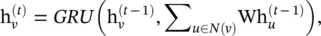

where . Unlike GNN and GraphESN, GGNN uses the backpropagation through time (BPTT) algorithm to learn the model parameters. This can be problematic for large graphs, as GGNN needs to run the recurrent function multiple times over all nodes, requiring the intermediate states of all nodes to be stored in memory.

Stochastic Steady‐state Embedding ( SSE ) uses a learning algorithm that is more scalable to large graphs [43]. It updates a node’s hidden states recurrently in a stochastic and asynchronous fashion. It alternatively samples a batch of nodes for state update and a batch of nodes for gradient computation. To maintain stability, the recurrent function of SSE is defined as a weighted average of the historical states and new states, which takes the form

(5.35)

where α is a hyperparameter, and is initialized randomly. Although conceptually important, SSE does not theoretically prove that the node states will gradually converge to fixed points by applying Eq. (5.35)repeatedly.

These networks are closely related to recurrent GNNs. Instead of iterating node states with contractive constraints, they address the cyclic mutual dependencies architecturally using a fixed number of layers with different weights in each layer, as illustrated in Figure 5.2a. This key distinction from recurrent GNNs is illustrated in Figures 5.2b and 5.2c. As graph convolutions are more efficient and convenient to composite with other neural networks, the popularity of ConvGNNs has been rapidly growing in recent years. These networks fall into two categories, spectral‐based and spatial‐based. Spectral‐based approaches define graph convolutions by introducing filters from the perspective of graph signal processing [44] where the graph convolutional operation is interpreted as removing noise from graph signals. Spatial‐based approaches inherit ideas from RecGNNs to define graph convolutions by information propagation. Since GCN [14] bridged the gap between spectral‐based approaches and spatial‐based approaches, spatial‐based methods have developed rapidly recently due to their attractive efficiency, flexibility, and generality.

Spectral ‐ based ConvGNNs assume graphs to be undirected. The normalized graph Laplacian matrix is a mathematical representation of an undirected graph, defined as 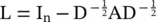, where D is a diagonal matrix of node degrees, D ii= ∑ j(A i, j). For details, see Appendix 5.A. The normalized graph Laplacian matrix possesses the property of being real symmetric positive semidefinite. With this property, the normalized Laplacian matrix can be factored as L = U Λ U T, where U = [u 0, u 1, ⋯, u n − 1] ∈ R n × nis the matrix of eigenvectors ordered by eigenvalues, and Λ is the diagonal matrix of eigenvalues (spectrum), Λ ii= λ i. The eigenvectors of the normalized Laplacian matrix form an orthonormal space, in mathematical words U TU= I. In graph signal processing, a graph signal x ∈ R nis a feature vector of all nodes of a graph where x iis the value of the i ‐th node. The graph Fourier transform to a signal x is defined as 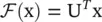, and the inverse graph Fourier transform is defined as 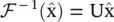, where represents the resulting signal from the graph Fourier transform. For more details, see Appendix 5.A. The graph Fourier transform projects the input graph signal to the orthonormal space where the basis is formed by eigenvectors of the normalized graph Laplacian. Elements of the transformed signal are the coordinates of the graph signal in the new space so that the input signal can be represented as which is exactly the inverse graph Fourier transform. Now, the graph convolution * Gof the input signal x with a filter g ∈ R nis defined as

(5.36)

where ⊙ denotes the element‐wise product. If we denote a filter as g θ= diag (U Tg), then the spectral graph convolution * Gis simplified as

(5.37)

Spectral‐based ConvGNNs all follow this definition. The key difference lies in the choice of the filter g θ.

Spectral Convolutional Neural Network ( Spectral CNN ) [12] assumes the filter is a set of learnable parameters and considers graph signals with multiple channels. The graph convolutional layer of Spectral CNN is defined as

(5.38)

where k is the layer index, is the input graph signal, H (0)= X, f k − 1is the number of input channels and f kis the number of output channels, and is a diagonal matrix filled with learnable parameters. Due to the eigen decomposition of the Laplacian matrix, spectral CNN faces three limitations: (i) any perturbation to a graph results in a change of eigenbasis; (ii) the learned filters are domain dependent, meaning they cannot be applied to a graph with a different structure; and (iii) eigen decomposition requires O ( n 3) computational complexity. In follow‐up works, ChebNet [45] and GCN [14, 46] reduced the computational complexity to O ( m ) by making several approximations and simplifications.