Savo G. Glisic - Artificial Intelligence and Quantum Computing for Advanced Wireless Networks

Neural Network for Graphs ( NN4G ) [48]: Proposed in parallel with GNN*, this is the first work toward spatial‐based ConvGNNs. Distinctively different from RecGNNs, NN4G learns graph mutual dependency through a compositional neural architecture with independent parameters at each layer. The neighborhood of a node can be extended through incremental construction of the architecture. NN4G performs graph convolutions by summing up a node’s neighborhood information directly. It also applies residual connections and skips connections to memorize information over each layer. As a result, NN4G derives its next layer node states by

(5.47)

where f (·) is an activation function and . The equation can also be written in a matrix form:

(5.48)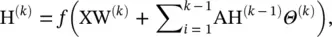

which resembles the form of GCN [14]. One difference is that NN4G uses the unnormalized adjacency matrix, which may potentially cause hidden node states to have extremely different scales.

Contextual Graph Markov Model ( CGMM ) [20] proposes a probabilistic model inspired by NN4G. While maintaining spatial locality, CGMM has the benefit of probabilistic interpretability

DCNN [16] regards graph convolutions as a diffusion process. It assumes that information is transferred from one node to one of its neighboring nodes with a certain transition probability so that information distribution can reach equilibrium after several rounds. DCNN defines the diffusion graph convolution (DGC) as

(5.49)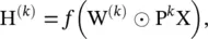

where f (·) is an activation function, and the probability transition matrix P ∈ R n × nis computed by P = D −1A. Note that in DCNN, the hidden representation matrix H (k)remains the same dimension as the input feature matrix X and is not a function of its previous hidden representation matrix H (k − 1). DCNN concatenates H (1), H (2), ⋯, H (K)together as the final model outputs. As the stationary distribution of a diffusion process is the sum of the power series of probability transition matrices, DGC [49] sums up outputs at each diffusion step instead of concatenating them. It defines the DGC by

(5.50)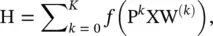

where W (k)∈ R D × Fand f (·) is an activation function. Using the power of a transition probability matrix implies that distant neighbors contribute very little information to a central node.

Parametric graph convolution (parametric GC ‐DGCNN) [12, 39] increases the contributions of distant neighbors based on shortest paths. It defines a shortest path adjacency matrix S (j). If the shortest path from a node v to a node u is of length j , then otherwise 0. With a hyperparameter r to control the receptive field size, PGC‐DGCNN introduces a graph convolutional operation as follows:

(5.51)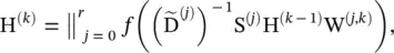

where 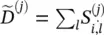, H (0)= X, and ‖ represents the concatenation of vectors. The calculation of the shortest path adjacency matrix can be expensive with O ( n 3) at maximum. An illustration of parameter r is given in Figure 5.4[39]

Partition graph convolution ( PGC ) [50] partitions a node’s neighbors into Q groups based on certain criteria not limited to shortest paths. PGC constructs Q adjacency matrices according to the defined neighborhood by each group. Then, PGC applies GCN [14] with a different parameter matrix to each neighbor group and sums the results:

(5.52)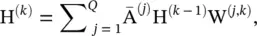

where 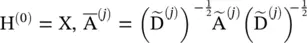and

MPNN [51] outlines a general framework of spatial‐based ConvGNNs. It treats graph convolutions as a message passing process in which information can be passed from one node to another along edges directly. MPNN runs K‐step message passing iterations to let information propagate further. The message passing function (namely the spatial graph convolution) is defined as

(5.53)

where =x v, U k(·) and M k(·) are functions with learnable parameters. After deriving the hidden representations of each node, can be passed to an output layer to perform node‐level prediction tasks or to a readout function to perform graph‐level prediction tasks. The readout function generates a representation of the entire graph based on node hidden representations. It is generally defined as

(5.54)

where R (·) represents the readout function with learnable parameters. MPNN can cover many existing GNNs by assuming different forms of U k(·), M k(·), and R (·).

Graph Isomorphism Network ( GIN) : Reference [52] finds that previous MPNN‐based methods are incapable of distinguishing different graph structures based on the graph embedding they produced. To amend this drawback, GIN adjusts the weight of the central node by a learnable parameter ε (k). It performs graph convolutions by

(5.55)