Savo G. Glisic - Artificial Intelligence and Quantum Computing for Advanced Wireless Networks

where z vis the embedding of node v . GAE* is trained by minimizing the negative cross‐entropy given the real adjacency matrix A and the reconstructed adjacency matrix

Simply reconstructing the graph adjacency matrix may lead to overfitting due to the capacity of the autoencoders. The variational graph autoencoder (VGAE) [56] is a variational version of GAE that was developed to learn the distribution of data. The VGAE optimizes the variational lower bound L :

(5.64)

where KL (·) is the Kullback–Leibler divergence function, which measures the distance between two distributions; p (Z) is a Gaussian prior , with q (z i∣ X, A) = N (z i∣ μ i, diag .

The mean vector μ iis the i ‐th row of an encoder’s outputs defined by Eq. (5.62), and log σ iis derived similarly as μ iwith another encoder. According to Eq. (5.64), VGAE assumes that the empirical distribution q (Z ∣ X, A) should be as close as possible to the prior distribution p (Z). To further enforce this, the empirical distribution q (Z ∣ X, A) is chosen to approximate the prior distribution p (Z).

Like GAE*, GraphSAGE [23] encodes node features with two graph convolutional layers. Instead of optimizing the reconstruction error, GraphSAGE shows that the relational information between two nodes can be preserved by negative sampling with the loss:

(5.65)

where node u is a neighbor of node v , node v nis a distant node to node v and is sampled from a negative sampling distribution P n( v ), and Q is the number of negative samples. This loss function essentially imposes similar representations on close nodes and dissimilar representations on distant nodes.

Deep Recursive Network Embedding ( DRNE ) [57] assumes that a node’s network embedding should approximate the aggregation of its neighborhood network embeddings. It adopts an LSTM network [26] to aggregate a node’s neighbors. The reconstruction error of DRNE is defined as

(5.66)

where z vis the network embedding of node v obtained by a dictionary look‐up, and the LSTM network takes a random sequence of node v ′s neighbors ordered by their node degree as inputs. As suggested by Eq. (5.66), DRNE implicitly learns network embeddings via an LSTM network rather than by using the LSTM network to generate network embeddings. It avoids the problem that the LSTM network is not invariant to the permutation of node sequences. Network representations with adversarially regularized autoencoders ( NetRA ) [58] proposes a graph encoder‐decoder framework with a general loss function, defined as

(5.67)

where dist (·) is the distance measure between the node embedding z and the reconstructed z. The encoder and decoder of NetRA are LSTM networks with random walks rooted on each node v ∈ V as inputs.

Graph generation (decoding) : With multiple graphs, GAEs are able to learn the generative distribution of graphs by encoding graphs into hidden representations and decoding a graph structure given the hidden representations. These methods either propose a new graph in a sequential manner or in a global manner.

Sequential approaches generate a graph by proposing nodes and edges step by step.

Deep Generative Model of Graphs ( DeepGMG ) [59] assumes that the probability of a graph is the sum over all possible node permutations:

(5.68)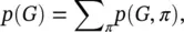

where π denotes a node ordering. It captures the complex joint probability of all nodes and edges in the graph. DeepGMG generates graphs by making a sequence of decisions, namely, whether to add a node, which node to add, whether to add an edge, and which node to connect to the new node. The decision process of generating nodes and edges is conditioned on the node states and the graph state of a growing graph updated by an RecGNN.

Global approaches output a graph all at once.

Graph variational autoencoder ( GraphVAE ) [60] models the existence of nodes and edges as independent random variables. By assuming the posterior distribution q φ(z∣ G ) defined by an encoder and the generative distribution p θ( G ∣ z) defined by a decoder, GraphVAE optimizes the variational lower bound:

(5.69)

where p (z) follows a Gaussian prior, φ and θ are learnable parameters. With a ConvGNN as the encoder and a simple multi‐layer perception as the decoder, GraphVAE outputs a generated graph with its adjacency matrix, node attributes, and edge attributes

These networks are designed to capture the dynamics of graphs. STGNNs follow two directions, recurrent neural network (RNN)‐based methods and CNN‐based methods. Most RNN‐based approaches capture spatial‐temporal dependencies by filtering inputs and hidden states passed to a recurrent unit using graph convolutions. To illustrate this (see Figure 5.7), suppose a simple RNN takes the form

(5.70)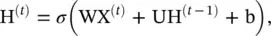

where X (t)∈ R n × dis the node feature matrix at time step t . After inserting graph convolution, Eq. (5.70)becomes

(5.71)