Savo G. Glisic - Artificial Intelligence and Quantum Computing for Advanced Wireless Networks

(5.74)

where l n, l co[n], x ne[n], and l ne[n]are the label of n , the labels of its edges, the states, and the labels of the nodes in the neighborhood of n , respectively.

Let x , o , l and l Nbe the vectors constructed by stacking all the states, all the outputs, all the labels, and all the node labels, respectively. Then, a compact form of Eq. (5.74)becomes

(5.75)

where F w, the global transition function , and G w, the global output function , are stacked versions of ∣ N ∣ instances of f wand g w, respectively. For us, the case of interest is when x , o are uniquely defined and Eq. (5.75)defines a map ϕ w: that takes a graph as input and returns an output o nfor each node. Banach’s fixed‐point theorem [62] provides a sufficient condition for the existence and uniqueness of the solution of a system of equations. According to Banach’s theorem, Eq. (5.75)has a unique solution provided that F wis a contraction map with respect to the state; that is, there exists μ , 0 ≤ μ < 1 such that ‖ F w( x , l ) − F w( y , l )‖ ≤ μ ‖ x − y ‖ holds for any x , y , where ‖ . ‖ denotes a vectorial norm. Thus, for the moment, let us assume that F wis a contraction map. Later, we will show that, in GNNs, this property is enforced by an appropriate implementation of the transition function.

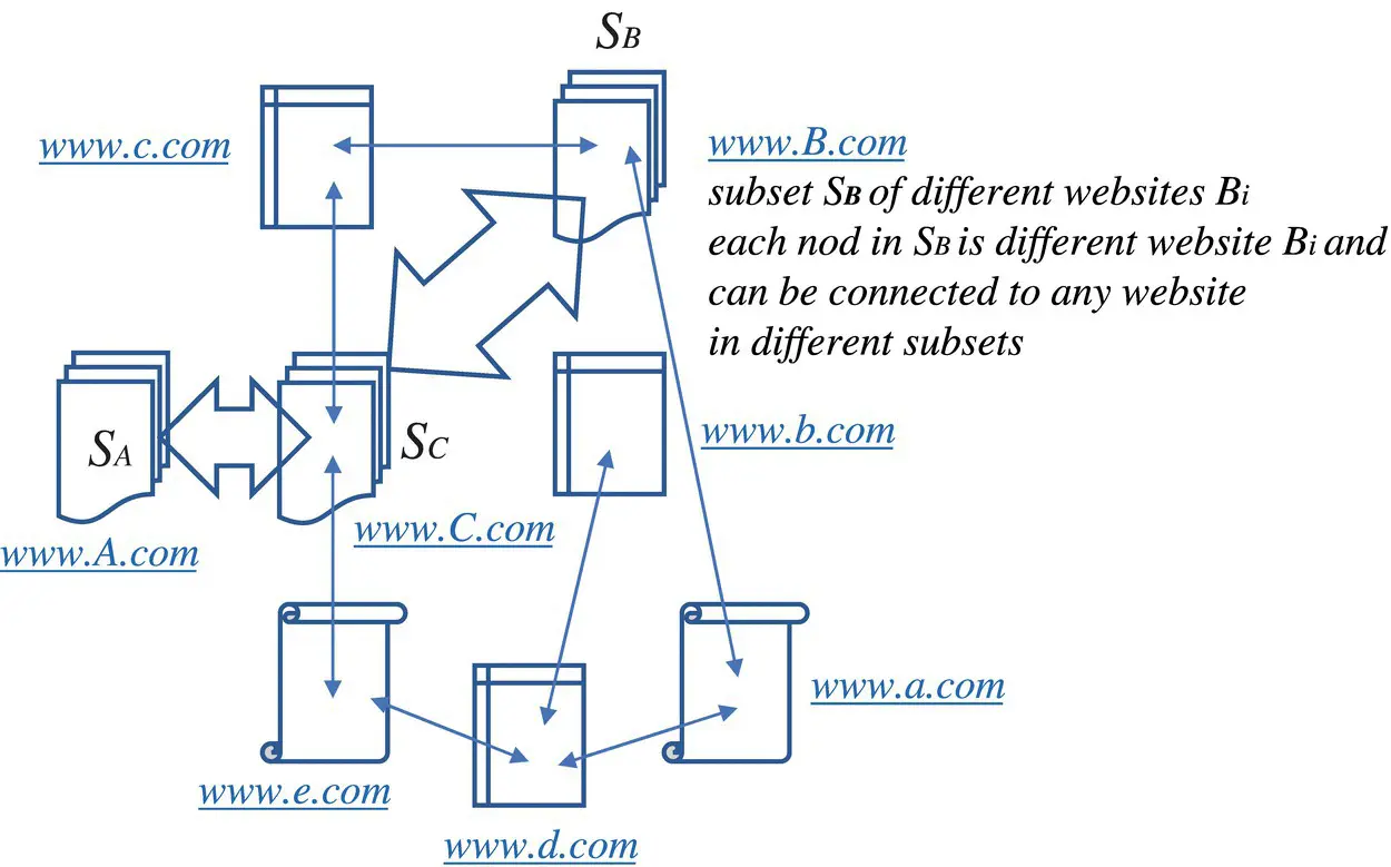
Figure 5.8 A subset of the Web.

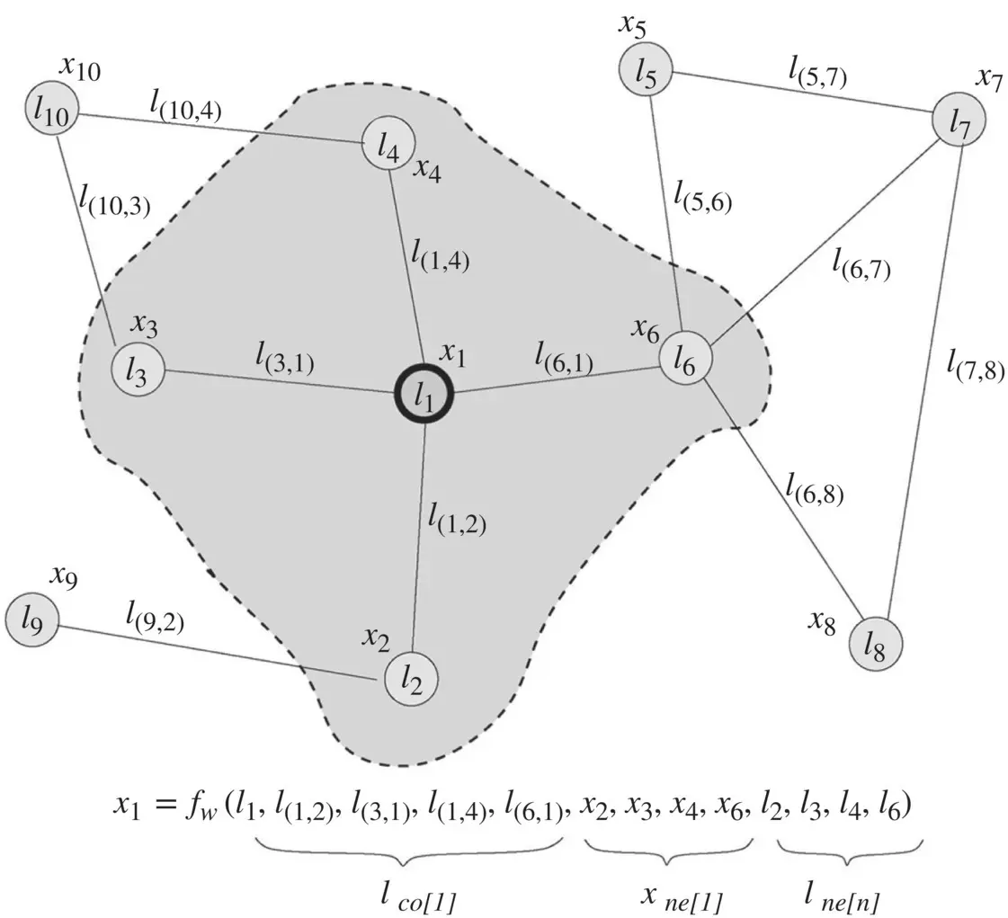
Figure 5.9 Graph and the neighborhood of a node. The state x 1of node 1 depends on the information contained in its neighborhood.

Source: Scarselli et al. [1].

For positional graphs , f wmust receive the positions of the neighbors as additional inputs. In practice, this can be easily achieved provided that information contained in x ne[n], l co[n], and l ne[n]is sorted according to neighbors’ positions and is appropriately padded with special null values in positions corresponding to nonexistent neighbors. For example, x ne[n]= [ y 1, …, y M], where M = max n, u v n( u ) is the maximum number of neighbors of a node; y i= x uholds, if u is the i ‐th neighbor of n ( ν n( u ) = i ); and y i= x 0, for some predefined null state x 0, if there is no i ‐th neighbor.

For nonpositional graphs , it is useful to replace function f wof Eq. (5.74)with

(5.76)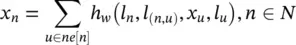

where h wis a parametric function. This transition function, which has been successfully used in recursive NNs, is not affected by the positions and the number of the children. In the following, Eq. (5.76)is referred to as the nonpositional form , and Eq. (5.74)is called the positional form . To implement the GNN model, we need (i) a method to solve Eq. (5.74)); (ii) a learning algorithm to adapt f wand g wusing examples from the training dataset; and (iii) an implementation of f wand g w. These steps will be considered in the following paragraphs.

Computation of the state : Banach’s fixed‐point theorem does not only ensure the existence and the uniqueness of the solution of Eq. (5.74), but it also suggests the following classic iterative scheme for computing the state:

(5.77)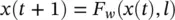

where x ( t ) denotes the t‐ th iteration of x . The dynamical system ( Eq. (5.77)) converges exponentially fast to the solution of Eq. (5.75)for any initial value (0). We can, therefore, think of x ( t ) as the state that is updated by the transition function F w. In fact, Eq. (5.77)implements the Jacobi iterative method for solving nonlinear equations [63]. Thus, the outputs and the states can be computed by iterating

(5.78)

Note that the computation described in Eq. (5.78)can be interpreted as the representation of a network consisting of units that compute f wand g w. Such a network is called an encoding network , following an analogous terminology used for the recursive neural network model [64]. In order to build the encoding network, each node of the graph is replaced by a unit computing the function f w(see Figure 5.10). Each unit stores the current state x n( t ) of node n , and when activated it calculates the state x n( t + 1) using the node label and the information stored in the neighborhood. The simultaneous and repeated activation of the units produce the behavior described in Eq. (5.78). The output of node n is produced by another unit, which implements g w. When f wand g ware implemented by FNNs, the encoding network turns out to be a recurrent neural network where the connections between the neurons can be divided into internal and external connections. The internal connectivity is determined by the neural network architecture used to implement the unit. The external connectivity depends on the edges of the processed graph.

The learning algorithm :Learning in GNNs consists of estimating the parameter w such that ϕ wapproximates the data in the learning dataset Eq. (5.73)where q iis the number of supervised nodes in G i. For graph‐focused tasks, one special node is used for the target ( q i= 1 holds), whereas for node‐focused tasks, in principle, the supervision can be performed on every node. The learning task can be posed as the minimization of a quadratic cost function

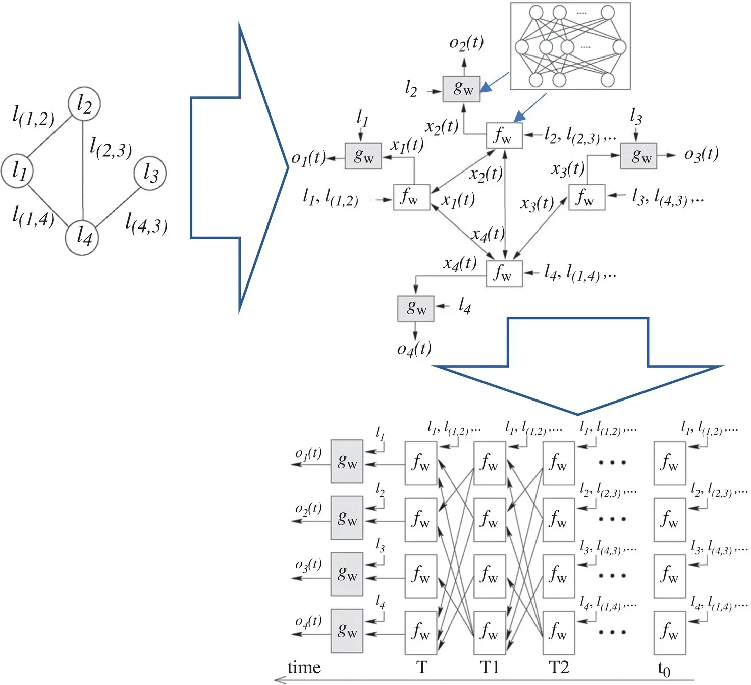
Figure 5.10 Graph (on the top, left), the corresponding encoding network (top right), and the network obtained by unfolding the encoding network (at the bottom).The nodes (the circles) of the graph are replaced, in the encoding network, by units computing f wand g w(the squares). When f wand g ware implemented by FNNs, the encoding network is a recurrent neural network. In the unfolding network, each layer corresponds to a time instant and contains a copy of all the units of the encoding network. Connections between layers depend on encoding network connectivity.