Savo G. Glisic - Artificial Intelligence and Quantum Computing for Advanced Wireless Networks

Table 5.1 [1] Learning algorithm.

The function FORWARD computes the states, whereas BACKWARD calculates the gradient. The procedure MAIN minimizes the error by calling FORWARD and BACKWARD iteratively.

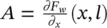
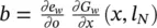
Note that in this case F w( x , l ) = Ax + b , where b is the vector constructed by stacking all the b n, and A is a block matrix , with if u is a neighbor of 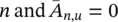otherwise. Vectors b nand matrices A n,udo not depend on the state x , but only on the node and edge labels. Thus, ∂F w/ ∂x = A , and, by simple algebra we have

which implies that F wis a contraction map (w.r. t. ‖ ‖ 1) for any set of parameters w .

1 Nonlinear (nonpositional) GNN. In this case, hw is realized by a multilayered feedforward NN. Since three‐layered neural networks are universal approximators [67], hw can approximate any desired function. However, not all the parameters w can be used, because it must be ensured that the corresponding transition function Fw is a contraction map. This can be achieved by adding a penalty term to Eq. (5.79), that is where the penalty term L(y) is (y − μ)2 if y > μ and 0 otherwise, and the parameter μ ∈ (0, 1) defines the desired contraction constant of Fw . More generally, the penalty term can be any expression, differentiable with respect to w, that is monotone increasing with respect to the norm of the Jacobian. For example, in our experiments, we use the penalty term , where Ai is the i‐th column of ∂Fw/∂x. In fact, such an expression is an approximation of L(‖∂Fw/∂x‖1) = L(maxi‖Ai‖1).

Here, we derive an analysis of the computational cost in GNN. The analysis will focus on three different GNN models: positional GNNs , where the functions f wand g wof Eq. (5.74)are implemented by FNNs; linear ( nonpositional ) GNNs ; and nonlinear ( nonpositional ) GNNs .

First, we will describe with more details the most complex instructions involved in the learning procedure (see Table 5.2reproduced from [1]). Then, the complexity of the learning algorithm will be defined. For the sake of simplicity, the cost is derived assuming that the training set contains just one graph G . Such an assumption does not cause any loss of generality, since the graphs of the training set can always be merged into a single graph. The complexity is measured by the order of floating point operations. By the common definition of time complexity, an algorithm requires O ( l ( a )) operations, if there exist α >0, , such that c ( a ) ≤ αl ( a ) holds for each , where c ( a ) is the maximal number of operations executed by the algorithm when the length of the input is a .

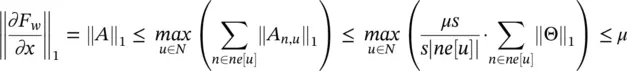
We will assume that there exist two procedures FP and BP, which implement the forward phase and the backward phase of the back propagation procedure, respectively. Formally, given a function l w: R a→ R bimplemented by an FNN, we have

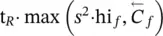
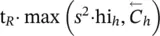
Table 5.2 Time complexity of the most expensive instructions of the learning algorithm. For each instruction and each GNN model, a bound on the order of floating point operations is given. The table also displays the number of times per epoch that each instruction is executed.

Source: Scarselli et al. [1].

Instruction	Positional	Nonlinear	Linear	Execs.
z ( t + 1) = z ( t ) ⋅ A + b	s 2∣ E ∣	s 2∣ E ∣	s 2∣ E ∣	it b
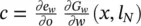
o = G w( x ( t ), l w)				1
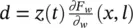
x ( t + 1) = F w( x ( t ), l )			s 2∣ E ∣	it f
				1
			–	1
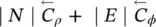
	∣ N ∣	∣ N ∣	∣ N ∣	1
			–	1
				1
				1
				1

Here, y ∈ R ais the input vector, and the row vector δ ∈ R bis a signal that suggests how the network output must be adjusted to improve the cost function. In most applications, the cost function is e w( y ) = ( t − y ) 2and δ =( ∂e w/ ∂o )( y ) = 2( t − o ), where o = l w( y ) and t (target) is the vector of the desired output corresponding to input y . On the other hand, δ ( ∂l w/ ∂y )( y ) is the gradient of e wwith respect to the network input and is easily computed as a side product of backpropagation. Backpropagation computes for each neuron v the delta value ( ∂e w/ ∂a v)( y ) = δ ( ∂l w/ ∂a v)( y ), where e wis the cost function and a vthe activation level of neuron v . Thus, δ ( ∂l w/ ∂y )( y ) is just a vector stacking all the delta values of the input neurons. Finally, denote the computational complexity required by the application of F P and BP on l w, respectively. For example, if l wis implemented by a multilayered FNN with a inputs, b hidden neurons, and c outputs, then 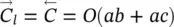holds.