Savo G. Glisic - Artificial Intelligence and Quantum Computing for Advanced Wireless Networks

Time complexity of the GNN model : Formally, the complexity is easily derived from Table 5.2: it is 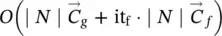for positional GNNs, 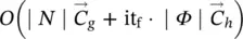for nonlinear GNNs, and for linear GNNs. In practice, the cost of the test phase is mainly due to the repeated computation of the state x ( t ). The cost of each iteration is linear with respect to both the dimension of the input graph (the number of edges) and the dimension of the employed FNNs and the state, with the sole exception of linear GNNs, whose single iteration cost is quadratic with respect to the state. The number of iterations required for the convergence of the state depends on the problem at hand, but Banach’s theorem ensures that the convergence is exponentially fast, and experiments have shown that 5–15 iterations are generally sufficient to approximate the fixed point [1].

In positional and nonlinear GNNs, the transition function must be activated it f· ∣ N ∣ and it f· ∣ E ∣ times, respectively. Even if such a difference may appear significant, in practice, the complexity of the two models is similar, because the network that implements the f wis larger than the one that implements h w. In fact, f whas M ( s + l E) input neurons, where M is the maximum number of neighbors for a node, whereas h whas only s + l Einput neurons. A significant difference can be noticed only for graphs where the number of neighbors of nodes is highly variable, since the inputs of f wmust be sufficient to accommodate the maximum number of neighbors, and many inputs may remain unused when f wis applied. On the other hand, it is observed that in the linear model the FNNs are used only once for each iteration, so that the complexity of each iteration is O ( s 2∣ E ∣) instead of . Note that holds, when h wis implemented by a three‐layered FNN with hi hhidden neurons. In practical cases, where hi his often larger than s , the linear model is faster than the nonlinear model. As confirmed by the experiments, such an advantage is mitigated by the smaller accuracy that the model usually achieves.

In GNNs, the learning phase requires much more time than the test phase, mainly due to the repetition of the forward and backward phases for several epochs. The experiments have shown that the time spent in the forward and backward phases is not very different. Similarly, to the forward phase, the cost of the function BACKWARD is mainly due to the repetition of the instruction that computes z ( t ). Theorem 5.2ensures that z ( t ) converges exponentially fast, and experiments have confirmed that it bis usually a small number.

Formally, the cost of each learning epoch is given by the sum of all the instructions times the iterations in Table 5.2. An inspection of the table shows that the cost of all instructions involved in the learning phase are linear with respect to both the dimension of the input graph and of the FNNs. The only exceptions are due to the computation of z ( t + 1) = z ( t ) · A + b , ( ∂F w/ ∂x )( x , l ) and ∂p w/ w , which depend quadratically on s.

The most expensive instruction is apparently the computation of ∂p w/ w in nonlinear GNNs, which costs O 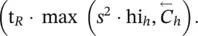On the other hand, the experiments have shown [1] that t Ris usually a small number. In most epochs, t Ris 0, since the Jacobian does not violate the imposed constraint, and in the other cases, t Ris usually in the range 1–5. Thus, for a small state dimension s , the computation of ∂p w/ w requires few applications of backpropagation on h and has a small impact on the global complexity of the learning process. On the other hand, in theory, if s is very large, it might happen that and at the same time t R≫ 0, causing the computation of the gradient to be very slow.

Let G = ( V , E ) be an undirected graph with vertex set V = { v 1, …, v n}. In the following, we assume that the graph G is weighted, that is, each edge between two vertices v iand v jcarries a non‐negative weight w ij≥ 0. The weighted adjacency matrix of the graph is the matrix W = ( w ij) i, j = 1, …, n. If w ij= 0, this means that the vertices v iand v jare not connected by an edge. As G is undirected, we require w ij= w ji. The degree of a vertex v i∈ V is defined as

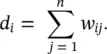
Note that, in fact, this sum only runs over all vertices adjacent to v i, as for all other vertices v jthe weight w ijis 0. The degree matrix D is defined as the diagonal matrix with the degrees d 1, …, d non the diagonal. Given a subset of vertices A ⊂ V , we denote its complement V \ A by . We define the indicator vector I A= ( f 1, …, f n)′ ∈ ℝ nas the vector with entries f i= 1 if v i∈ A and f i= 0 otherwise. For convenience, we introduce the shorthand notation i ∈ A for the set of indices { i ∣ v i∈ A }, in particular when dealing with a sum like ∑ i ∈ A w ij. For two not necessarily disjoint sets A , B ⊂ V we define

We consider two different ways of measuring the “ size” of a subset ⊂ A :

Intuitively, ∣ A ∣ measures the size of A by its number of vertices, whereas vol( A ) measures the size of A by summing over the weights of all edges attached to vertices in A . A subset A ⊂ V of a graph is connected if any two vertices in A can be joined by a path such that all intermediate points also lie in A . A subset A is called a connected component if it is connected and if there are no connections between vertices in A and . The nonempty sets A 1, …, A kform a partition of the graph if A i∩ A j= ∅ and A 1∪ … ∪ A k= V .