Savo G. Glisic - Artificial Intelligence and Quantum Computing for Advanced Wireless Networks

Directed Laplacian : As discussed in Appendix 5.A, the graph Laplacian for undirected graphs is a symmetric difference operator L=D − W, where D is the degree matrix of the graph, and W is the weight matrix of the graph. In the case of directed graphs (or digraphs), the weight matrix W of a graph is not symmetric. In addition, the degree of a vertex can be defined in two ways: in‐degree and out‐degree. The in‐degree of a node i is estimated as , whereas the out‐degree of the node i can be calculated as 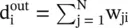. We consider an in‐degree matrix and define the directed Laplacian L of a graph as

(5.B.1)

where D in= diag is the in‐degree matrix. Figure 5.B.1shows an example of weighted directed graph, with the corresponding matrices [68]. The Laplacian for a directed graph is not symmetric; nevertheless, it follows some important properties: (i) the sum of each row is zero, and hence λ = 0 is certainly an eigenvalue, and (ii) real parts of the eigenvalues are non‐negative for a graph with positive edge weights.

Figure 5.B.1 A directed graph and the corresponding matrices.

Graph Fourier transform based on directed Laplacian : Using Jordan decomposition, the graph Laplacian is decomposed as

(5.B.2)

where J, known as the Jordan matrix, is a block diagonal matrix similar to L, and the Jordan eigenvectors of L constitute the columns of V. We define the graph Fourier transform (GFT) of a graph signal f as

(5.B.3)

Here, V is treated as the graph Fourier matrix whose columns constitute the graph Fourier basis. The inverse graph Fourier transform can be calculated as

(5.B.4)

In this definition of GFT, the eigenvalues of the graph Laplacian act as the graph frequencies, and the corresponding Jordan eigenvectors act as the graph harmonics. The eigenvalues with a small absolute value correspond to low frequencies and vice versa. Before discussing the ordering of frequencies, we consider a special case when the Laplacian matrix is diagonalizable.

Diagonalizable Laplacian matrix: When the graph Laplacian is diagonalizable, Eq. (5.B.2)is reduced to

(5.B.5)

Here, Λ ∈ ℂ N × Nis a diagonal matrix containing the eigenvalues λ 0, λ 1, …, λ N − 1of L, and V = [v 0, v 1, …, v N − 1] ∈ ℂ N × Nis the matrix with columns as the corresponding eigenvectors of L. Note that for a graph with real non‐negative edge weights, the graph spectrum will lie in the right half of the complex frequency plane (including the imaginary axis).

Undirected graphs : For an undirected graph with real weights, the graph Laplacian matrix L is real and symmetric. As a result, the eigenvalues of L turn out to be real, and L constitutes orthonormal set of eigenvectors. Hence, the Jordan form of the Laplacian matrix for undirected graphs can be written as

(5.B.6)

where V T= V −1, because the eigenvectors of L are orthogonal in th undirected case. Consequently, the GFT of a signal f can be given as , and the inverse can be calculated as f=V . One can show that for the example from Figure 5.B.1for the signal f = [0.12 0.38 0.81 0.24 0.88] we have the GFT as

1 1 Scarselli, F., Gori, M., Tsoi, A.C. et al. (2009). The graph neural network model. IEEE Trans. Neural Netw. 20 (1): 61–80.

2 2 Khamsi, M.A. and Kirk, W.A. (2011). An Introduction to Metric Spaces and Fixed Point Theory, vol. 53. Wiley.

3 3 M. Kampffmeyer, Y. Chen, X. Liang, H. Wang, Y. Zhang, and E. P. Xing, “Rethinking knowledge graph propagation for zero‐shot learning,” arXiv preprint arXiv:1805.11724, 2018.

4 4 Y. Zhang, Y. Xiong, X. Kong, S. Li, J. Mi, and Y. Zhu, “Deep collective classification in heterogeneous information networks,” in WWW 2018, 2018, pp. 399–408.

5 5 X. Wang, H. Ji, C. Shi, B. Wang, Y. Ye, P. Cui, and P. S. Yu, “Heterogeneous graph attention network,” WWW 2019, 2019.

6 6 D. Beck, G. Haffari, and T. Cohn, “Graph‐to‐sequence learning using gated graph neural networks,” in ACL 2018, 2018, pp. 273–283.

7 7 M. Schlichtkrull, T. N. Kipf, P. Bloem, R. van den Berg, I. Titov, and M. Welling, “Modeling relational data with graph convolutional networks,” in ESWC 2018. Springer, 2018, pp. 593–607

8 8 Y. Li, R. Yu, C. Shahabi, and Y. Liu, “Diffusion convolutional recurrent neural network: Data‐driven traffic forecasting,” arXiv preprint arXiv:1707.01926, 2017.

9 9 B. Yu, H. Yin, and Z. Zhu, “Spatio‐temporal graph convolutional networks: A deep learning framework for traffic forecasting,” arXiv preprint arXiv:1709.04875, 2017. 20

10 10 A. Jain, A. R. Zamir, S. Savarese, and A. Saxena, “Structural‐rnn: Deep learning on spatio‐temporal graphs,” in CVPR 2016, 2016, pp. 5308–5317.

11 11 S. Yan, Y. Xiong, and D. Lin, “Spatial temporal graph convolutional networks for skeleton‐based action recognition,” in Thirty Second AAAI Conference on Artificial Intelligence, 2018.

12 12 J. Bruna, W. Zaremba, A. Szlam, and Y. Lecun, “Spectral networks and locally connected networks on graphs,” ICLR 2014, 2014.

13 13 Hammond, D.K., Vandergheynst, P., and Gribonval, R. (2011). Wavelets on graphs via spectral graph theory. Appl. Comput. Harmonic Anal. 30 (2): 129–150.

14 14 T. N. Kipf and M. Welling, “Semi‐supervised classification with graph convolutional networks,” in Proc. of ICLR 2017, 2017.