Savo G. Glisic - Artificial Intelligence and Quantum Computing for Advanced Wireless Networks

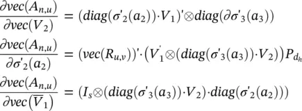
where d his the number of hidden neurons. Then, we have

(5.87)

(5.88)

(5.89)

(5.90)

where the aforementioned Kronecker product properties have been used.

It follows that (vec ( R u,v)) ′· ∂vec( A n,u)/ ∂w can be written as the sum of the four contributions represented by Eqs. (5.87)– (5.90). The second and the fourth terms – Eqs. (5.88)and (5.90)– can be computed directly using the corresponding formulas. The first one can be calculated by observing that looks like the function computed by a three‐layered FNN that is the same as h wexcept for the activation function of the last layer. In fact, if we denote by such a network, then

(5.91)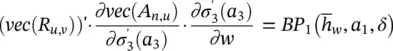

holds, where . A similar reasoning can be applied also to the third contribution.

Required number of operations: The above method includes two tasks: the matrix multiplications of Eqs. (5.87)– (5.90)and the backpropagation as defined by Eq. (5.91). The former task consists of several matrix multiplications. By inspection of Eqs. (5.87)– (5.90), the number of floating point operations is approximately estimated as 2 s 2+ 12 s hi h+ 10 s 2· hi h, where hi hdenotes the number of hidden‐layer neurons implementing the function h . The second task has approximately the same cost as a backpropagation phase through the original function h w. Such a value is obtained from the following observations: for an a × b matrix C and a b × c matrix D , the multiplication CD requires approximately 2 abc operations; more precisely, abc multiplications and ac ( b − 1) sums. If D is a diagonal b × b matrix, then CD requires 2 ab operations. Similarly, if C is an a × b matrix, D is a b × a matrix, and P ais the a 2× a matrix defined above and used in Eqs. (5.87)– (5.90), then computing vec( CD ) P ccosts only 2 ab operations provided that a sparse representation is used for P α. Finally, a 1, a 2, a 3are already available, since they are computed during the forward phase of the learning algorithm. Thus, the complexity of computing ∂p w/ ∂w is 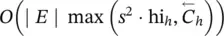. Note, however, that even if the sum in Eq. (5.85)ranges over all the arcs of the graph, only those arcs ( n , u ) such that R n, u≠ 0 have to be considered. In practice, R n, u≠ 0 is a rare event, since it happens only when the columns of the Jacobian are larger than μ , and a penalty function was used to limit the occurrence of these cases. As a consequence, a better estimate of the complexity of computing ∂p w/ ∂w is O 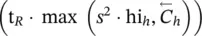, where t Ris the average number of nodes u such that R n, u≠ 0 holds for some n .

1 Instructions b = (∂ew/∂o)(∂Gw/∂x)(x, lN) and =(∂ew/∂o)(∂Gw/∂w)(x, lN): The terms b and c can be calculated by the backpropagation of ∂ew/∂o through the network that implements gw . Since such an operation must be repeated for each node, the time complexity of instructions b = (∂ew/∂o)(∂Gw/∂x)(x, lN) and c = (∂ew/∂o)(∂Gw/∂w)(x, lN) is for all the GNN models.

2 Instruction = z(t)(∂Fw/∂w)(x, l): By definition of Fw, fw , and BP, we have(5.92)

where y = [ l n, x u, l (n, u), l u] and BP 1indicates that we are considering only the first part of the output of BP. Similarly

(5.93)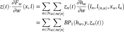

where y = [ l n, x u, l (n, u), l u]. These two equations provide a direct method to compute d in positional and nonlinear GNNs, respectively.

For linear GNNs, let denote the the output of h wand note that

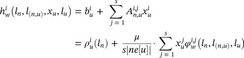
holds where and are the element in position i , j of matrix A n, uand the corresponding output of the transition network, respectively, while is the the element of vector is the corresponding output of the forcing network (see Eq. (5.83))], and is the i ‐th element of x u. Then

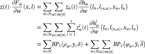
where y 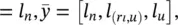δ = ∣ ne[ n ] ∣ · z ′( t ), and is a vector that stores in the position corresponding to i , j , that is, . Thus, in linear GNNs, d is computed by calling the backpropagation procedure on each arc and node.