Savo G. Glisic - Artificial Intelligence and Quantum Computing for Advanced Wireless Networks

(4.17)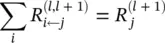

must hold. In the case of a linear network f ( x ) = ∑ i z ijwhere the relevance R j= f ( x ), such a decomposition is immediately given by R i ← j= z ij. However, in the general case, the neuron activation x jis a nonlinear function of z j. Nevertheless, for the hyperbolic tangent and the rectifying function – two simple monotonically increasing functions satisfying g (0) = 0‐the pre‐activations z ijstill provide a sensible way to measure the relative contribution of each neuron x ito R j. A first possible choice of relevance decomposition is based on the ratio of local and global pre‐activations and is given by

(4.18)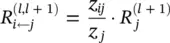

These relevances R i ← jare easily shown to approximate the conservation properties, in particular:

(4.19)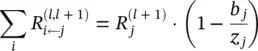

where the multiplier accounts for the relevance that is absorbed (or injected) by the bias term. If necessary, the residual bias relevance can be redistributed onto each neuron x i. A drawback of the propagation rule of Eq. (4.18)is that for small values z j, relevances R j ← jcan take unbounded values. Unboundedness can be overcome by introducing a predefined stabilizer ε ≥ 0:

(4.20)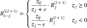

The conservation law then becomes

(4.21)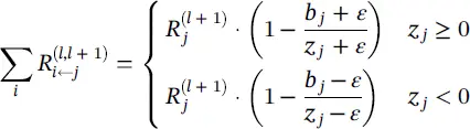

where we can observe that some further relevance is absorbed by the stabilizer. In particular, relevance is fully absorbed if the stabilizer ε becomes very large.

An alternative stabilizing method that does not leak relevance consists of treating negative and positive pre‐activations separately. Let 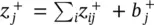and 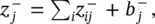where – and + denote the negative and positive parts of z ijand b j. Relevance propagation is now defined as

(4.22)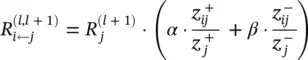

where α + β = 1. For example, for αβ = 1/2, the conservation law becomes

(4.23)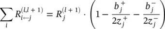

which has a similar form as Eq. (4.19). This alternative propagation method also allows one to manually control the importance of positive and negative evidence, by choosing different factors α and β .

Once a rule for relevance propagation has been selected, the overall relevance of each neuron in the lower layer is determined by summing up the relevances coming from all upper‐layer neurons in agreement with Eqs. (4.8)and (4.9):

(4.24)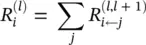

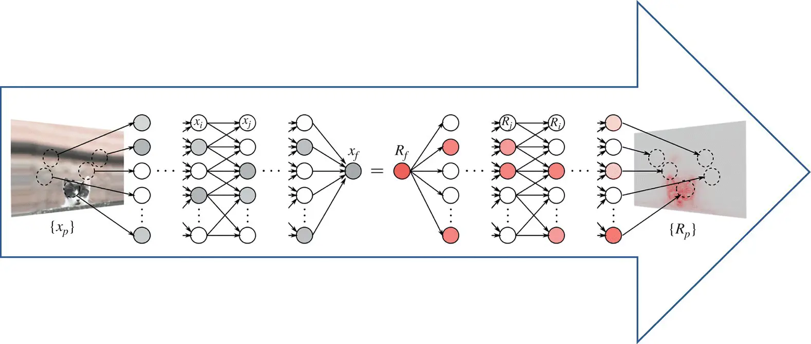
Figure 4.3 Relevance propagation (heat map; relevance is presented by the intensity of the red color).

Source: Montavon et al. [92].

The relevance is backpropagated from one layer to another until it reaches the input pixels x (d), and where the relevances provide the desired pixel‐wise decomposition of the decision f ( x ). A practical example of relevance propagation obtained by Deep Taylor decomposition is shown in Figure 4.3[92].

In this section, we consider long short term memory networks (LSTMs), which were discussed in Chapter 3, and described an approach for tracking the importance of a given input to the LSTM for a given output. By identifying consistently important patterns of words, we are able to distill state‐of‐the‐art LSTMs on sentiment analysis and question answering into a set of representative phrases. This representation is then quantitatively validated by using the extracted phrases to construct a simple rule‐based classifier that approximates the output of the LSTM.

Word importance scores in LSTMS: Here, we present a decomposition of the output of an LSTM into a product of factors, where each term in the product can be interpreted as the contribution of a particular word. Thus, we can assign importance scores to words according to their contribution to the LSTM’s prediction. We have introduced the basics of LSTM networks in the Chapter 3. Given a sequence of word embeddings x 1, x T∈ ℝ d, an LSTM processes one word at a time, keeping track of cell and state vectors ( c 1, h 1), ( c T, h T), which contain information in the sentence up to word i . h tand c tare computed as a function of x t, c t − 1using the updates given by Eq. (3.72)of Chapter 3, which we repeat here with slightly different notation:

(4.25)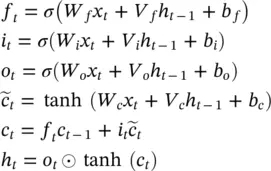

As initial values, we define c 0= h 0= 0. After processing the full sequence, a probability distribution over C classes is specified by p , with

(4.26)

where W iis the i ‐th row of the matrix W .

Decomposing the output of an LSTM: We now decompose the numerator of p iin Eq. (4.26)into a product of factors and show that we can interpret those factors as the contribution of individual words to the predicted probability of class i . Define

(4.27)