Savo G. Glisic - Artificial Intelligence and Quantum Computing for Advanced Wireless Networks

(4.4)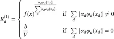

This clearly satisfies Eqs. (4.1)and (4.2); however, the relevances R (1)( x d) of all input dimensions have the same sign as the prediction f ( x ). In terms of pixel‐wise decomposition interpretation, all inputs point toward the presence of a structure if f ( x ) > 0 and toward the absence of a structure if f ( x ) < 0. This is for many classification problems not a realistic interpretation. As a solution, for this example we define an alternative

(4.5)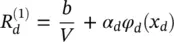

Then, the relevance of a feature dimension x ddepends on the sign of the term in Eq. (4.5). This is for many classification problems a more plausible interpretation. This second example shows that LRP is able to deal with nonlinearities such as the feature space mapping φ dto some extent and how an example of LRP satisfying Eq. (4.2)may look like in practice.

The above example gives an intuition about what relevance R is, namely, the local contribution to the prediction function f ( x ). In that sense, the relevance of the output layer is the prediction itself: f ( x ). This first example shows what one could expect as a decomposition for the linear case. The linear case is not a novelty; however, it provides a first intuition. A more graphic and nonlinear example is given in Figure 4.1. The upper part of the figure shows a neural‐network‐shaped classifier with neurons and weights w ijon connections between neurons. Each neuron i has an output a ifrom an activation function.The top layer consists of one output neuron, indexed by 7. For each neuron i we would like to compute a relevance R i. We initialize the top layer relevance as the function value; thus, . LRP in Eq. (4.2)requires now to hold

(4.6)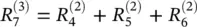

(4.7)

We will make two assumptions for this example. First, we express the layer‐wise relevance in terms of messages between neurons i and j which can be sent along each connection. The messages are, however, directed from a neuron toward its input neurons, in contrast to what happens at prediction time, as shown in the lower part of Figure 4.1. Second, we define the relevance of any neuron except neuron 7 as the sum of incoming messages ( k : i is input for neuron k ):

(4.8)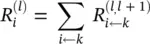

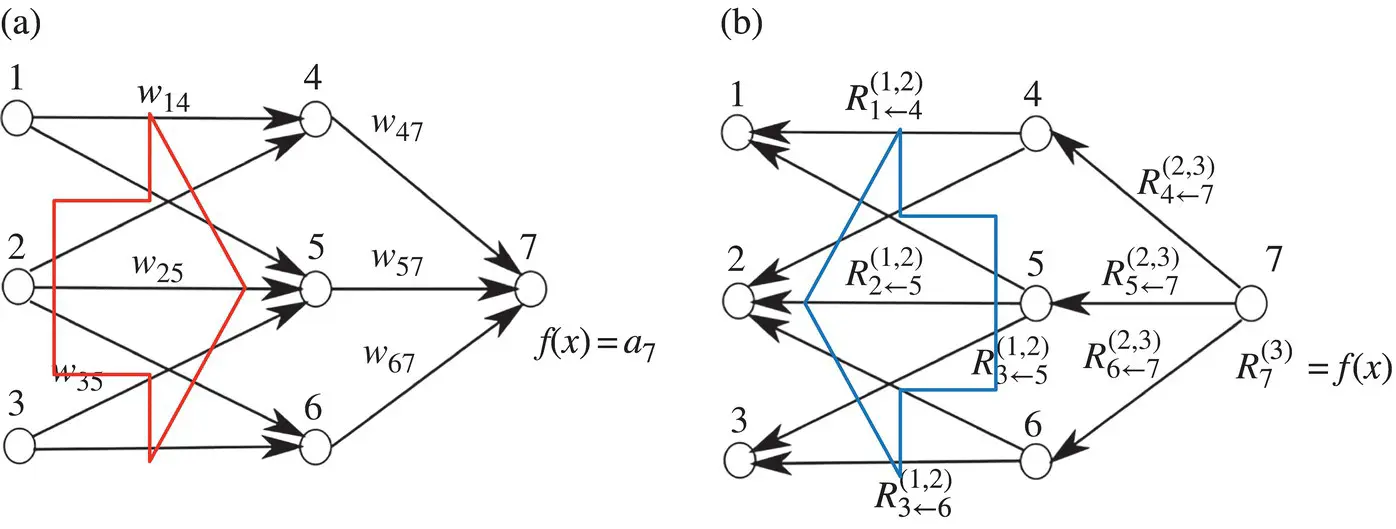
Figure 4.1 (a) Neural network (NN) as a classifier, (b) NN during the relevance computation.

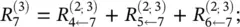
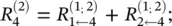
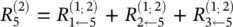
For example, 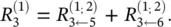Note that neuron 7 has no incoming messages anyway. Instead, its relevance is defined as . In Eq. (4.8)and the following text, the terms input and source have the meaning of being an input to another neuron in the direction defined during the time of classification, not during the time of computation of LRP. For example in Figure 4.1, neurons 1 and 2 are the inputs and source for neuron 4, while neuron 6 is the sink for neurons 2 and 3. Given the two assumptions encoded in Eq. (4.8), the LRP by Eq. (4.2)can be satisfied by the following sufficient condition:

and 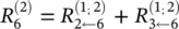. In general, this condition can be expressed as

(4.9)

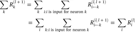
The difference between condition (4.9)and definition (4.8)is that in condition (4.9)the sum runs over the sources at layer l for a fixed neuron k at layer l + 1, whereas in definition (4.8)the sum runs over the sinks at layer l + 1 for a fixed neuron i at a layer l . When using Eq. (4.8)to define the relevance of a neuron from its messages, then condition (4.9)is a sufficient condition I order to ensure that Eq. (4.2)holds. Summing over the left hand side in Eq. (4.9)yields

One can interpret condition (4.9)by saying that the messages are used to distribute the relevance of a neuron k onto its input neurons at layer l . In the following sections, we will use this notion and the more strict form of relevance conservation as given by definition (4.8)and condition (4.9). We set Eqs. (4.8)and (4.9)as the main constraints defining LRP. A solution following this concept is required to define the messages according to these equations.