Savo G. Glisic - Artificial Intelligence and Quantum Computing for Advanced Wireless Networks

Now we can derive an explicit formula for LRP for our example by defining the messages . The LRP should reflect the messages passed during classification time. We know that during classification time, a neuron i inputs a i w ikto neuron k , provided that i has a forward connection to k . Thus, we can rewrite expressions for and so that they match the structure of the right‐hand sides of the same equations by the following:

(4.10)

(4.11)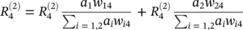

The match of the right‐hand sides of the initial expressions for and against the right‐hand sides of Eqs. (4.10)and (4.11)can be expressed in general as

(4.12)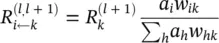

Although this solution, Eq. (4.12), for message terms still needs to be adapted such that it is usable when the denominator becomes zero, the example given in Eq. (4.12)gives an idea of what a message could be, namely, the relevance of a sink neuron that has been already computed, weighted proportionally by the input of neuron i from the preceding layer l .

Taylor‐type decomposition: An alternative approach for achieving a decomposition as in Eq. (4.1)for a general differentiable predictor f is a first‐order Taylor approximation:

(4.13)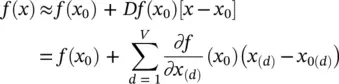

The choice of a Taylor base point x 0is a free parameter in this setup. As stated above, in the case of classification, we are interested in finding out the contribution of each pixel relative to the state of maximal uncertainty of the prediction given by the set of points f ( x 0) = 0, since f ( x ) > 0 denotes the presence and f ( x ) < 0 denotes the absence of the learned structure. Thus, x 0should be chosen to be a root of the predictor f . Thus, the above equation simplifies to

(4.14)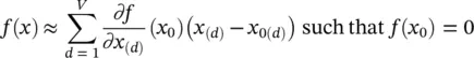

The pixel‐wise decomposition contains a nonlinear dependence on the prediction point x beyond the Taylor series, as a close root point x 0needs to be found. Thus, the whole pixel‐wise decomposition is not a linear, but a locally linear algorithm, as the root point x 0depends on the prediction point x .

Pixel‐wise decomposition for multilayer networks: In the previous chapter, we discussed NN networks built as a set of interconnected neurons organized in a layered structure. They define a mathematical function when combined with each other that maps the first‐layer neurons (input) to the last‐layer neurons (output). In this section, we denote each neuron by x i, where i is an index for the neuron. By convention, we associate different indices for each layer of the network. We denote by ∑ ithe summation over all neurons of a given layer, and by ∑ jthe summation over all neurons of another layer. We denote by x (d)the neurons corresponding to the pixel activations (i.e., with which we would like to obtain a decomposition of the classification decision). A common mapping from one layer to the next one consists of a linear projection followed by a nonlinear function: z ij= x j w ij, z j= ∑ i z ij+ b j, x j= g ( z j), where w ijis a weight connecting neuron x ito neuron x j, b jis a bias term, and g is a nonlinear activation function. Multilayer networks stack several of these layers, each of them being composed of a large number of neurons. Common nonlinear functions are the hyperbolic tangent g ( t ) = tanh ( t ) or the rectification function g ( t ) = max (0, t )

Taylor‐type decomposition: Denoting by f : ℝ M↦ ℝ Nthe vector‐valued multivariate function implementing the mapping between input and output of the network, a first possible explanation of the classification decision x ↦ fx ) can be obtained by Taylor expansion at a near root point x 0of the decision function f :

(4.15)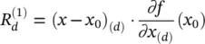

The derivative ∂fx )/ ∂x (d)required for pixel‐wise decomposition can be computed efficiently by reusing the network topology using the backpropagation algorithm discussed in the previous chapter. Having backpropagated the derivatives up to a certain layer j , we can compute the derivative of the previous layer i using the chain rule:

(4.16)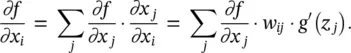

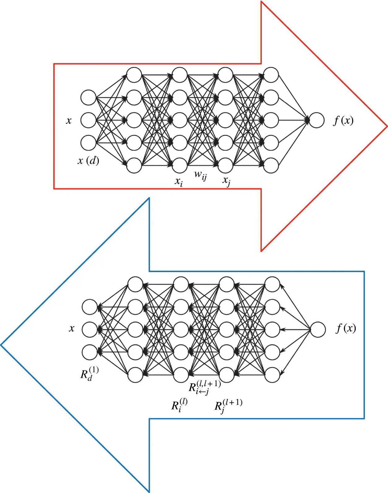
Figure 4.2 Relevance propagation.

Layer‐wise relevance backpropagation: As an alternative to Taylor‐type decomposition, it is possible to compute relevances at each layer in a backward pass, that is, express relevances as a function of upper‐layer relevances , and backpropagating relevances until we reach the input (pixels). Figure 4.2depicts a graphic example. The method works as follows: Knowing the relevance of a certain neuron for the classification decision f ( x ), one would like to obtain a decomposition of this relevance in terms of the messages sent to the neurons of the previous layers. We call these messages R i ← j. As before, the conservation property