Savo G. Glisic - Artificial Intelligence and Quantum Computing for Advanced Wireless Networks

(3.81)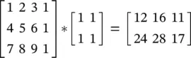

where the first matrix is denoted as A , and * is the convolution operator.

The MATLAB command B = im2col(A, [2 2]) gives the B matrix, which is an expanded version of A:

(3.82)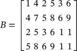

Note that the first column of B corresponds to the first 2 × 2 region in A , in a column‐first order, corresponding to ( i l + 1, j l + 1) = (0, 0). Similarly, the second to last column in B correspond to regions in A with ( i l + 1, j l + 1) being (1, 0), (0, 1), (1, 1), (0, 2) and (1, 2), respectively. That is, the MATLAB im2col function explicitly expands the required elements for performing each individual convolution to create a column in the matrix B . The transpose, B T, is called the im2row expansion of A . If we vectorize the convolution kernel itself into a vector (in the same column‐first order) (1, 1, 1, 1) T, we find that

(3.83)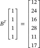

If we reshape this resulting vector properly, we get the exact convolution result matrix in Eq. (3.81).

If D l> 1 ( x lhas more than one channel, e.g., in Figure 3.24of RGB image/three channels), the expansion operator could first expand the first channel of x l, then the second, … , until all D lchannels are expanded. The expanded channels will be stacked together; that is, one row in the im2row expansion will have H × W × D lelements, rather than H × W .

Suppose x lis a third‐order tensor in , with one element in x lrepresented by ( i l, j l, d l), and f is a set of convolution kernels whose spatial extent are all H × W . Then, the expansion operator (im2row) converts x linto a matrix φ( x l) with elements indexed as ( p , q ). The expansion operator copies the element at ( i l, j l, d l) in x lto the ( p , q )‐th entry in φ( x l). From the description of the expansion process, given a fixed ( p , q ), we can calculate its corresponding ( i l, j l, d l) triplet from the relation

(3.84)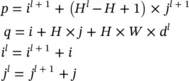

As an example, dividing q by HW and take the integer part of the quotient, we can determine which channel ( d l) belongs to.

We can use the standard vec operator to convert the set of convolution kernels f (an order‐4 tensor) into a matrix. Starting from one kernel, which can be vectorized into a vector in , all convolution kernels can be reshaped into a matrix with HWD lrows and D columns with D l+1= D referred to as matrix F . With these notations, we have an expression to calculate convolution results (in Eq. (3.83), φ( x l) is B T):

(3.85)

with 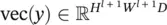, φ( x l) 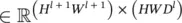, and 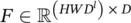. The matrix multiplication φ( x l) F results in a matrix of size ( H l + 1 W l + 1) × D . The vectorization of this resultant matrix generates a vector in , which matches the dimensionality of vec( y ).

The Kronecker product : Given two matrices A ∈ ℝ m × nand B ∈ ℝ p × q, the Kronecker product A ⊗ B is a mp × nq matrix, defined as a block matrix

(3.86)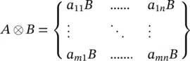

The Kronecker product has the following properties that will be useful for us:

(3.87)

(3.88)

The last equation can be utilized from both directions. Now we can write down

(3.89)

(3.90)

where I is an identity matrix of appropriate size. In Eq. (3.89), the size of I is determined by the number of columns in F , and hence I ∈ ℝ D × D. In Eq. (3.90), For the derivation of the gradient computation rules in a convolution layer, the notation summarized in Table 3.3will be used.

Update the parameters – backward propagation: First, we need to compute ∂z /∂vec( x l) and z /∂vec( F ), where the first term will be used for backward propagation to the previous ( l − 1)th layer, and the second term will determine how the parameters of the current ( l −th) layer will be updated. Keep in mind that f , F , and w irefer to the same thing (modulo reshaping of the vector or matrix or tensor). Similarly, we can reshape y into a matrix ; then y , Y , and x l + 1refer to the same object (again, modulo reshaping).