Savo G. Glisic - Artificial Intelligence and Quantum Computing for Advanced Wireless Networks

Then, we can use the “indicator” method to encode the function m ( p , q ) = ( i l, j l, d l) into M . That is, for any possible element in M , its row index x determines a( p , q ) pair, and its column index y determines a( i l, j l, d l) triplet, and M is defined as

(3.95)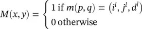

The M matrix is very high dimensional. At the same time, it is also very sparse: there is only one nonzero entry in the H l W l D lelements in one row, because m is a function. M , which uses information [A, B, C.1], encodes only the one‐to‐one correspondence between any element in φ( x l) and any element in x l; it does not encode any specific value in x l. Putting together the one‐to‐one correspondence information in M and the value information in x l, we have

(3.96)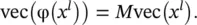

Supervision signal for the previous layer : In the l ‐th layer, we need to compute ∂z /∂vec( x l). For that, we want to reshape x linto a matrix , and use these two equivalent forms (modulo reshaping) interchangeably. By the chain rule, ∂z / ∂ (vec( x l) T) = [ ∂z / ∂ (vec( y ) T)][∂vec( y )/ ∂ (vec( x l) T)].

By utilizing Eqs. (3.90)and (3.96), we have

(3.97)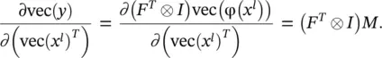

(3.98)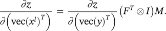

Since by using Eq. (3.88)

(3.99)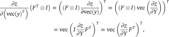

we have

(3.100)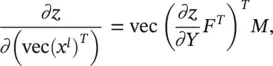

or equivalently

(3.101)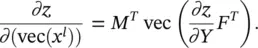

In Eq. (3.101), , and vec(( ∂z / ∂Y ) F T) is a vector in . At the same time, M Tis an indicator matrix in In order to locate one element in vec( x l) or one row in M T, we need an index triplet ( i l, j l, d l), with 0 ≤ i l< H l, 0 ≤ j l< W l, and 0 ≤ d l< D l. Similarly, to locate a column in M Tor an element in ∂z / ∂Y ) F T, we need an index pair p , q ), with 0≤ p < H l + 1 W l + 1and ≤ q < HW D l. Thus, the ( i l, j l, d l)‐th entry of ∂z / ∂ (vec( x l)) is the product of two vectors: the row in M T(or the column in M ) that is indexed by ( i l, j l, d l), and vec(( ∂z / ∂Y ) F T). Since M Tis an indicator matrix, in the row vector indexed by ( i l, j l, d l), only those entries whose index ( p , q ) satisfies m ( p , q ) = ( i l, j l, d l) have a value 1, and all other entries are 0. Thus, the ( i l, j l, d l)‐th entry of ∂z / ∂ (vec( x l)) equals the sum of these corresponding entries in vec(( ∂z / ∂Y ) F T). Therefore, we get the following succinct equation:

(3.102)

In other words, to compute ∂z / ∂X , we do not need to explicitly use the extremely high‐dimensional matrix M . Instead, Eqs. (3.102)and (3.84)can be used to efficiently find it. The convolution example from Figure 3.23is used to illustrate the inverse mapping m −1in Figure 3.25.

In the right half of Figure 3.25, the 6 × 4 matrix is ∂z / ∂Y ) F T. In order to compute the partial derivative of z with respect to one element in the input X , we need to find which elements in ∂z / ∂Y ) F Tare involved and add them. In the left half of Figure 3.25, we see that the input element 5 (shown in larger font) is involved in four convolution operations, shown by the gray, light gray, dotted gray and black boxes, respectively. These four convolution operations correspond to p = 1, 2, 3, 4. For example, when p = 2 (the light gray box), 5 is the third element in the convolution, and hence q = 3 when p = 2, and we put a light gray circle in the (2, 3)‐th element of the ( ∂z / ∂Y ) F Tmatrix. After all four circles are put in the matrix ( ∂z / ∂Y ) F T,the partial derivative is the sum of ellements in these four locations of ( ∂z / ∂Y ) F T. The set m −1( i l, j l, d l) contains at most HWD lelements. Hence, Eq. (3.102)requires at most HWD lsummations to compute one element of ∂z / ∂X .

The pooling layer : Let be the input to the l ‐th layer, which is now a pooling layer. The pooling operation requires no parameter (i.e., w iis null, and hence parameter learning is not needed for this layer). The spatial extent of the pooling ( H × W ) is specified in the design of the CoNN structure. Assume that H divides H land W divides W land the stride equals the pooling spatial extent, the output of pooling ( y or equivalently x l + 1) will be an order‐3 tensor of size H l + 1× W l + 1× D l + 1, with H l + 1= H l/ H , W l + 1= W l/ W , D l + 1= D l. A pooling layer operates upon x lchannel by channel independently. Within each channel, the matrix with H l× W lelements is divided into H l + 1× W l + 1nonoverlapping subregions, each subregion being H × W in size. The pooling operator then maps a subregion into a single number. Two types of pooling operators are widely used: max pooling and average pooling. In max pooling, the pooling operator maps a subregion to its maximum value, while the average pooling maps a subregion to its average value as illustrated in Figure 3.26.