Savo G. Glisic - Artificial Intelligence and Quantum Computing for Advanced Wireless Networks

(3.79)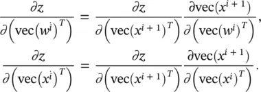

Since ∂z / ∂x i + 1is already computed and stored in memory, it requires just a matrix reshaping operation (vec) and an additional transpose operation to get ∂z / ∂ (vec( x i + 1) T). As long as we can compute ∂vec( x i + 1)/ ∂ (vec( w i) T) and vec( x i + 1)/ ∂ (vec( x i) T), we can easily get Eq. (3.79). The terms ∂vec( x i + 1)/ ∂ (vec( w i) T) and ∂vec( x i + 1)/ ∂ (vec( x i) T) are much easier to compute than directly computing ∂z / ∂ (vec( w i) T) and ∂vec( x i + 1)/ ∂ (vec( x i) T) because x iis directly related to x i + 1through a function with parameters w i. The details of these partial derivatives will be discussed in the following sections.

Suppose we are considering the l ‐th layer, whose inputs form an order‐3 tensor x lwith . A triplet index set ( i l, j l, d l) is used to locate any specific element in x l. The triplet ( i l, j l, d l) refers to one element in x l, which is in the d l‐th channel, and at spatial location ( i l, j l) (at the i lth row, and j l‐th column). In actual CoNN learning, the mini‐batch strategy is usually used. In that case, x lbecomes an order‐4 tensor in , where N is the mini‐batch size. For simplicity we assume for the moment that N = 1. The results in this section, however, are easy to adapt to mini‐batch versions. In order to simplify the notations that will appear later, we follow the zero‐based indexing convention, which specifies that 0 ≤ i l< H l, 0 ≤ j l< W l, and 0 ≤ d l< D l. In the l ‐th layer, a function will transform the input x lto an output = x l + 1. We assume the output has size H l + 1× W l + 1× D l + 1, and an element in the output is indexed by a triplet ( i l + 1, j l + 1, d l + 1), 0 ≤ i l + 1< H l + 1, 0 ≤ j l + 1< W l + 1, 0 ≤ d l + 1< D l + 1.

The Rectified Linear Unit (ReLU) layer : An ReLU layer does not change the size of the input; that is, x land y share the same size. The ReLU can be regarded as a truncation performed individually for every element in the input: with 0 ≤ i < H l= H l + 1, 0 ≤ j < W l= W l + 1, and 0 ≤ d < D l= D l + 1. There is no parameter inside a ReLU layer, and hence there is no need for parameter learning in this layer.

The convolution layer: Figure 3.23illustrates a convolution of the input image (3 × 4 matrix) and the convolution kernel of size 2 × 2. For order‐3 tensors, the convolution operation is defined similarly. Figure 3.24illustrates an RGB (black/light gray/gray) image with three channels and three kernels. Suppose the input in the l ‐th layer is an order‐3 tensor of size H l× W l× D l. A convolution kernel is also an order‐3 tensor of size H × W × D l. When we overlap the kernel on top of the input tensor at the spatial location (0, 0, 0), we compute the products of the corresponding elements in all the D lchannels and sum the HWD lproducts to get the convolution result at this spatial location. Then, we move the kernel from top to bottom and from left to right to complete the convolution. In a convolution layer, multiple convolution kernels are usually used. Assuming D kernels are used and each kernel is of spatial span H × W, we denote all the kernels as f . f is an order‐4 tensor in . Similarly, we use index variables 0 ≤ i < H , 0 ≤ j < W , 0 ≤ d l< D land 0 ≤ d < D to pinpoint a specific element in the kernels.

Stride is another important concept in convolution. At the bottom of Figure 3.23, we convolve the kernel with the input at every possible spatial location, which corresponds to the stride s = 1. However, if s > 1, every movement of the kernel skips s − 1 pixel locations (i.e., the convolution is performed once every s pixels both horizontally and vertically). In this section, we consider the simple case when the stride is 1 and no padding is used. Hence, we have y (or x l + 1) in , with H l + 1= H l− H + 1, W l + 1= W l− W + 1, and D l + 1= D . For mathematical rigor, the convolution procedure can be expressed as an equation:

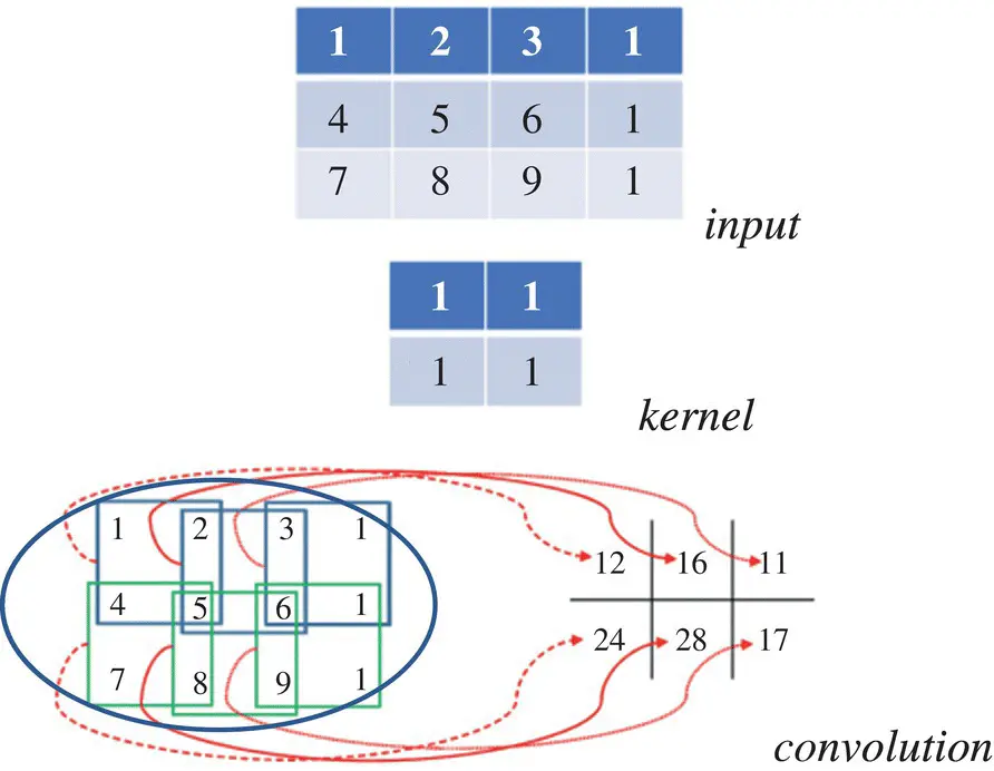
Figure 3.23 Illustration of the convolution operation. If we overlap the convolution kernel on top of the input image, we can compute the product between the numbers at the same location in the kernel and the input, and we get a single number by summing these products together. For example, if we overlap the kernel with the top‐left region in the input, the convolution result at that spatial location is 1 × 1 + 1 × 4 + 1 × 2 + 1 × 5 = 12. (for more details see the color figure in the bins).

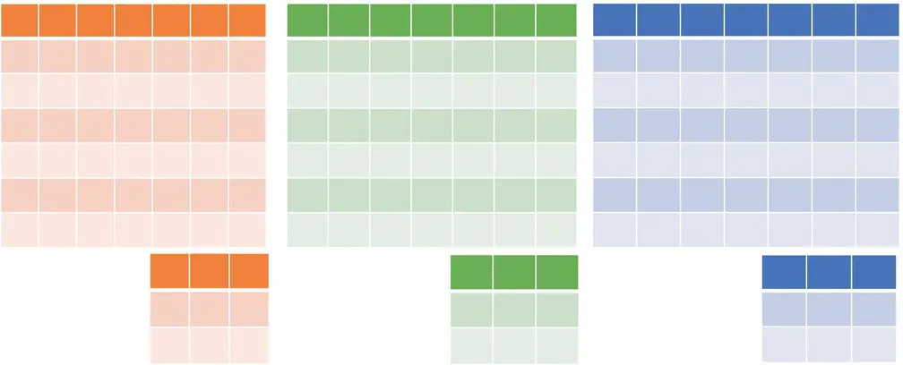
Figure 3.24 RGB image/three channels and three kernels. (for more details see the color figure in the bins).

(3.80)

Convolution as matrix product : There is a way to expand x land simplify the convolution as a matrix product. Let us consider a special case with D l= D = 1, H = W = 2, and H l= 3, W l= 4. That is, we consider convolving a small single‐channel 3 × 4 matrix (or image) with one 2 × 2 filter. Using the example in Figure 3.23, we have