Savo G. Glisic - Artificial Intelligence and Quantum Computing for Advanced Wireless Networks

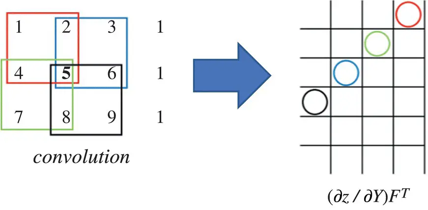
Figure 3.25 Computing ∂z / ∂X . (for more details see the color figure in the bins).

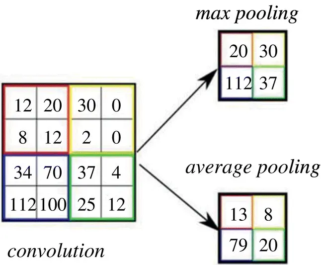
Figure 3.26 Illustration of pooling layer operation. (for more details see the color figure in the bins).

Formally this can be represented as

(3.103)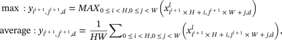

where 0 ≤ i l + 1< H l + 1, 0 ≤ j l + 1< W l + 1, and 0 ≤ d < D l + 1= D l.

Pooling is a local operator, and its forward computation is straightforward. When focusing on the backpropagation, only max pooling will be discussed and we can resort to the indicator matrix again. All we need to encode in this indicator matrix is: for every element in y , where does it come from in x l?

We need a triplet ( i l, j l, d l) to locate one element in the input x l, and another triplet ( i l + 1, j l + 1, d l + 1) to locate one element in y . The pooling output comes from , if and only if the following conditions are met: (i) they are in the same channel; (ii) the ( i l, j l)‐th spatial entry belongs to the ( i l + 1, j l + 1)‐th subregion; and (iii) the ( i l, j l)‐th spatial entry is the largest one in that subregion. This can be represented as

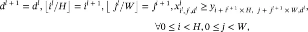
where ⌊·⌋ is the floor function. If the stride is not H ( W ) in the vertical (horizontal) direction, the equation must be changed accordingly. Given a ( i l + 1, j l + 1, d l + 1) triplet, there is only one ( i l, j l, d l) triplet that satisfies all these conditions. So, we define an indicator matrix .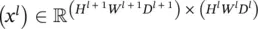

One triplet of indexes ( i l + 1, j l + 1, d l + 1) specifies a row in S , while ( i l, j l, d l) specifies a column. These two triplets together pinpoint one element in ( x l). We set that element to 1 if d l + 1= d land , are simultaneously satisfied, and 0 otherwise. One row of S ( x l) corresponds to one element in y , and one column corresponds to one element in x l. By using this indicator matrix, we have vec( y ) = S ( x l) vec ( x l) and

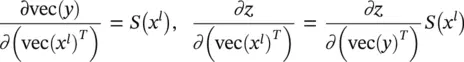
Figure 3.27 Illustration of preprocessing in a cooperative neural network (CoNN)‐based image classifier.

resulting in

(3.104)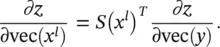

S ( x l) is very sparse since it has only one nonzero entry in every row. Thus, we do not need to use the entire matrix in the computation. Instead, we just need to record the locations of those nonzero entries – there are only H l + 1 W l + 1 D l + 1such entries in S ( x l). Figure 3.27illustrates preprocessing in a CoNN‐based image classifier.

For further readings on CoNNs, the reader is referred to [30].

1 1 CS231n Convolutional Neural Networks for Visual Recognition. Stanford University. https://cs231n.github.io/neural‐networks‐1

2 2 Haykin, S. (1996). Adaptive Filter Theory, 3e. Upper Saddle River, NJ: Prentice‐Hall.

3 3 Haykin, S. (1996). Neural networks expand SP's horizons. IEEE Signal Process. Mag. 13 (2): 24–49.

4 4 Haykin, S. (1999). Neural Networks: A Comprehensive Foundation, 2e. Upper Saddle River, NJ: Prentice‐Hall.

5 5 Wan, E.A. (1993). Finite impulse response neural networks with applications in time series prediction, Ph.D. dissertation. Department of Electrical Engineering, Stanford University, Stanford, CA.

6 6 Box, G. and Jenkins, G.M. (1976). Time Series Analysis: Forecasting and Control. San Francisco, CA: Holden‐Day.

7 7 Weigend, A.S. and Gershenfeld, N.A. (1994). Time Series Prediction: Fore‐ Casting the Future and Understanding the Past. Reading, MA: Addison‐Wesley.

8 8 Hochreiter, S. and Schmidhuber, J. (1997). Long short‐term memory. Neural Comput. 9 (8): 1735–1780.

9 9 Schuster, M. and Paliwal, K.K. (1997). Bidirectional recurrent neural networks. IEEE Trans. Signal Process. 45 (11): 2673–2681.

10 10 Graves, A. and Schmidhuber, J. (2005). Framewise phoneme classification with bidirectional LSTM and other neural network architectures. Neural Netw. 18 (5): 602–610.

11 11 Graves, A., Liwicki, M., Fernandez, S. et al. (2009). A novel connectionist system for unconstrained handwriting recognition. IEEE Trans. Pattern Anal. Mach. Intell. 31 (5): 855–868.

12 12 Graves, A., Wayne, G., and Danihelka, I. (2014). Neural Turing machines. arXiv preprint arXiv:1410.5401.

13 13 Baddeley, A., Sala, S.D., and Robbins, T.W. (1996). Working memory and executive control [and discussion]. Philos. Trans. R. Soc. B: Biol. Sci. 351 (1346): 1397–1404.

14 14 Chua, L.O. and Roska, T. (2002). Cellular Neural Networks and Visual Computing: Foundations and Applications. New York, NY: Cambridge University Press.

15 15 Chua, L.O. and Yang, L. (1988). Cellular neural network: theory. IEEE Trans. Circuits Syst. 35: 1257–1272.

16 16 Molinar‐Solis, J.E., Gomez‐Castaneda, F., Moreno, J. et al. (2007). Programmable CMOS CNN cell based on floating‐gate inverter unit. J. VLSI Signal Process. Syst. Signal, Image, Video Technol. 49: 207–216.

17 17 Pan, C. and Naeemi, A. (2016). A proposal for energy‐efficient cellular neural network based on spintronic devices. IEEE Trans. Nanotechnol. 15 (5): 820–827.

18 18 Wang, L. et al. (1998). Time multiplexed color image processing based on a CNN with cell‐state outputs. IEEE Trans. VLSI Syst. 6 (2): 314–322.

19 19 Roska, T. and Chua, L.O. (1993). The CNN universal machine: an analogic array computer. IEEE Trans. Circuits Systems II: Analog Digital Signal Process. 40 (3): 163–173.