Savo G. Glisic - Artificial Intelligence and Quantum Computing for Advanced Wireless Networks

The symmetry between the forward propagation of states and the backward propagation of error terms is preserved in temporal backpropagation. The number of operations per iteration now grows linearly with the number of layers and synapses in the network. This savings is due to the efficient recursive formulation. Each coefficient enters into the calculation only once, in contrast to the redundant use of terms when applying standard backpropagation to the unfolded network.

As an illustration of the computations involved, we consider a simple network consisting of only two segments (cascaded linear FIR filters shown in Figure 3.8). The first segment is defined as

(3.35)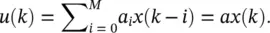

For simplicity, the second segment is limited to only three taps:

(3.36)

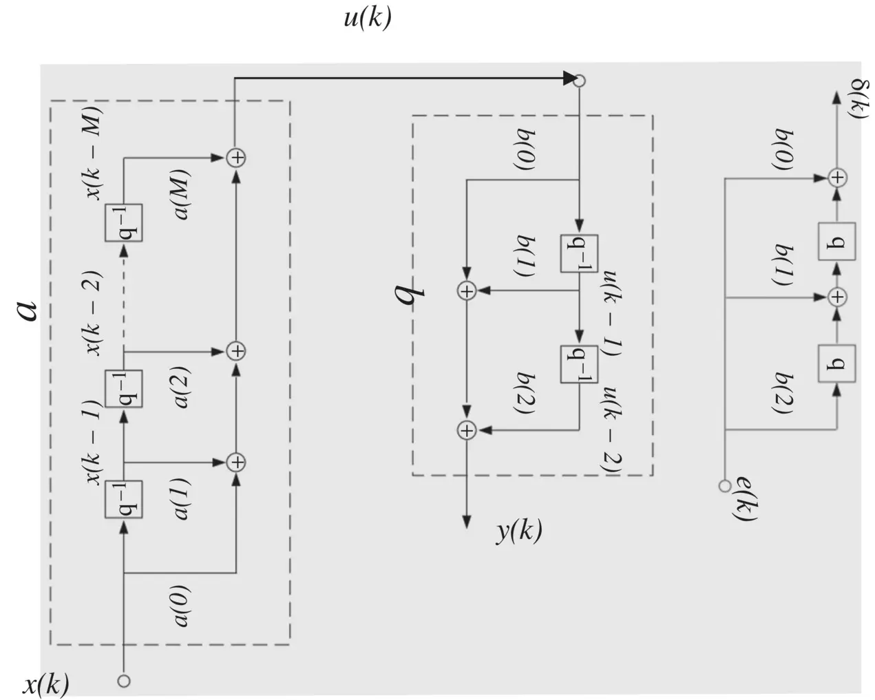
Figure 3.8 Oversimplified finite impulse response (FIR) network.

Here ( a is the vector of filter coefficient and should not be confused with the variable for the activation value used earlier). To adapt the filter coefficients, we evaluate the gradients ∂e 2( k )/ ∂a and ∂e 2( k )/ ∂b . For filter b , the desired response is available directly at the output of the filter of interest and the gradient is which yields the standard LMS update Δ b ( k ) = 2 μe ( k ) u ( k ). For filter a, we have

(3.37)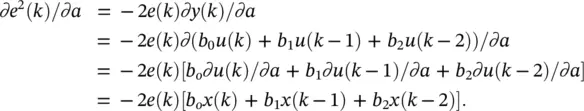

which yields

(3.38)

Here, approximately 3 M multiplications are required at each iteration of this update, which is the product of the orders of the two filters. This computational inefficiency corresponds to the original approach of unfolding a network in time to derive the gradient. However, we observe that at each iteration this weight update is repeated. Explicitly writing out the product terms for several iterations, we get

Iteration	Calculation
k	e ( k )	[		+	b 1 x( k − 1)	+	b 2 x( k − 2)	]
k + 1	e ( k + 1)	[	b o x( k + 1)	+		+	b 2 x( k − 1)	]
k + 2	e ( k + 2)	[	b o x( k + 2)	+	b 1 x( k − 1)	+		]
k + 3	e ( k + 3)	[	b o x( k + 3)	+	b 1 x( k − 2)	+	b 2 x( k + 1)	]

Therefore, rather than grouping along the horizontal in the above equations, we may group along the diagonal (boxed terms). Gathering these terms, we get

(3.39)

where δ ( k ) is simply the error filtered backward through the second cascaded filter as illustrated in Figure 3.8. The alternative weight update is thus given by

(3.40)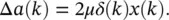

Equation (3.40)represents temporal backpropagation. Each update now requires only M + 3 multiplications, the sum of the two filter orders. So, we can see that a simple reordering of terms results into a more efficient algorithm. This is the major advantage of the temporal backpropagation algorithm.

In general, here we deal with the problem of predicting future samples of a time series using a number of samples from the past [6, 7]. Given M samples of the series, autoregression (AR) is fit to the data as

(3.41)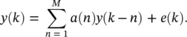

The model assumes that y ( k ) is obtained by summing up the past values of the sequence plus a modeling error e ( k ). This error represents the difference between the actual series y ( k ) and the single‐step prediction

(3.42)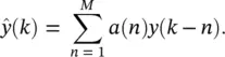

In nonlinear prediction, the model is based on the following nonlinear AR:

(3.43)

where g is a nonlinear function. The model can be used for both scalar and vector sequences. The one time step prediction can be represented as

(3.44)

Given the focus of this chapter, we discuss how the network models studied so far can be used when the inputs to the network correspond to the time window y ( k − 1) through ( k − M ). Using neural networks for predictions in this case has become increasingly popular. For our purposes, g will be realized with an FIR network. Thus, the prediction corresponding to the output of an FIR network with input y ( k − 1) can be represented as