Savo G. Glisic - Artificial Intelligence and Quantum Computing for Advanced Wireless Networks

where ω u,iand ω v,iare the weights associated with u and v , respectively. In the case of Figure 3.13b, we have

(3.64)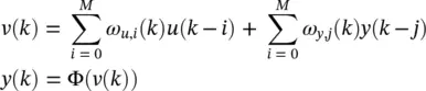

where ω y, jare the weights associated with the delayed outputs. The previous networks exhibit a locally recurrent structure, but when connected into a larger network, they have a feedforward architecture and are referred to as locally recurrent–globally feedforward ( LRGF ) architectures. A general LRGF architecture is shown in Figure 3.14. It allows dynamic synapses to be included within both the input (represented by H 1, … , H M) and the output feedback (represented by H FB), some of the aforementioned schemes. Some typical examples of these networks are shown in Figures 3.15– 3.18.

The following equations fully describe the RNN from Figure 3.17

(3.65)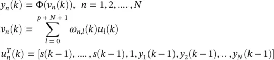

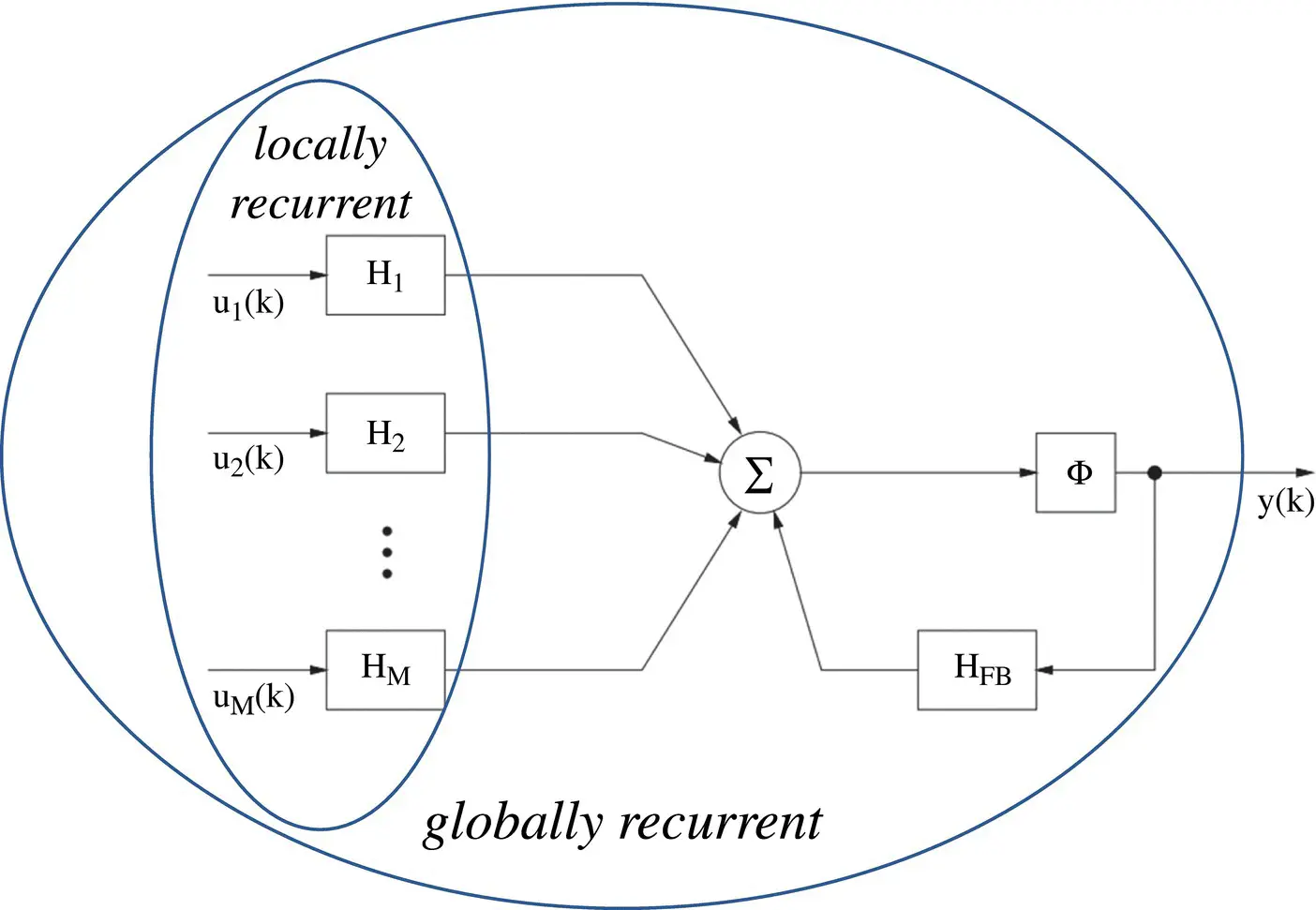
Figure 3.14 General locally recurrent–globally feedforward (LRGF) architecture.

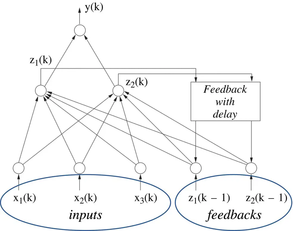
Figure 3.15 An example of Elman recurrent neural network (RNN).

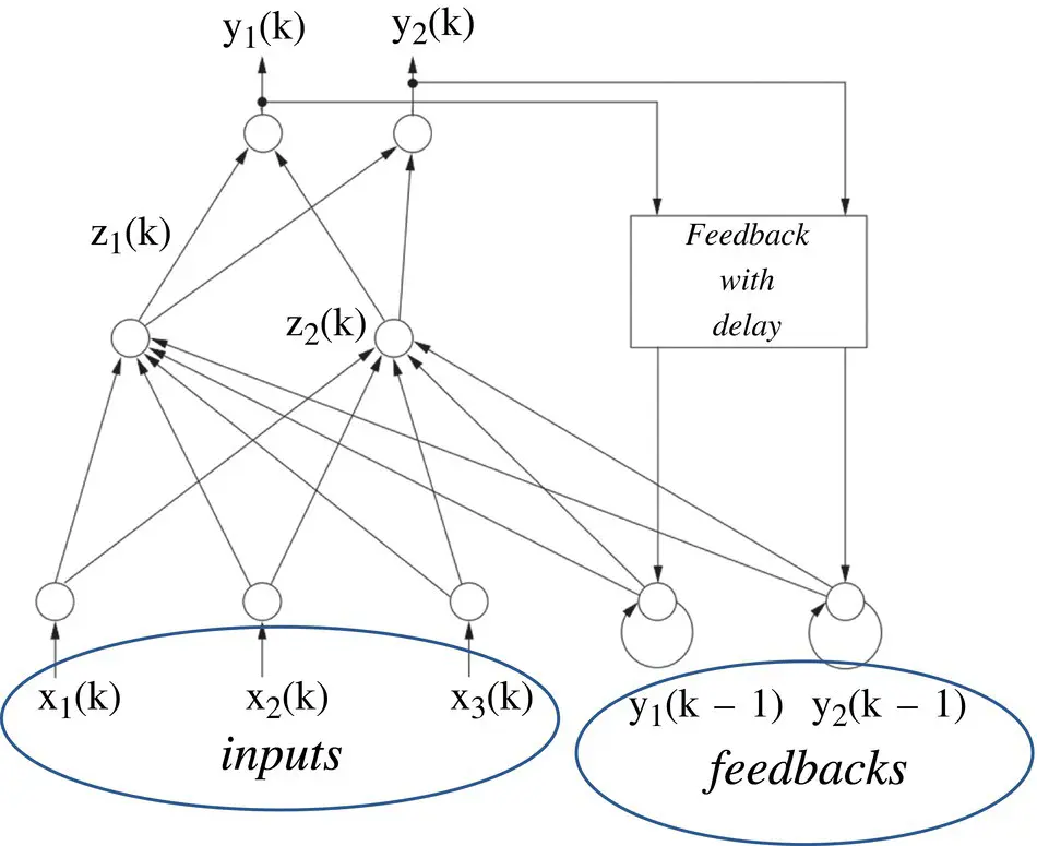
Figure 3.16An example of Jordan recurrent neural network (RNN).

where the (p + N + 1) × 1 dimensional vector u comprises both the external and feedback inputs to a neuron, as well as the unity valued constant bias input.

Training: Here, we discuss training the single fully connected RNN shown in Figure 3.17. The nonlinear time series prediction uses only one output neuron of the RNN. Training of the RNN is based on minimizing the instantaneous squared error at the output of the first neuron of the RNN which can be expressed as

(3.66)

where e(k) denotes the error at the output y1 of the RNN, and s(k) is the training signal. Hence, the correction for the l‐ th weight of neuron k at the time instant k is

(3.67)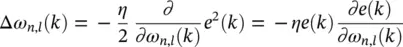

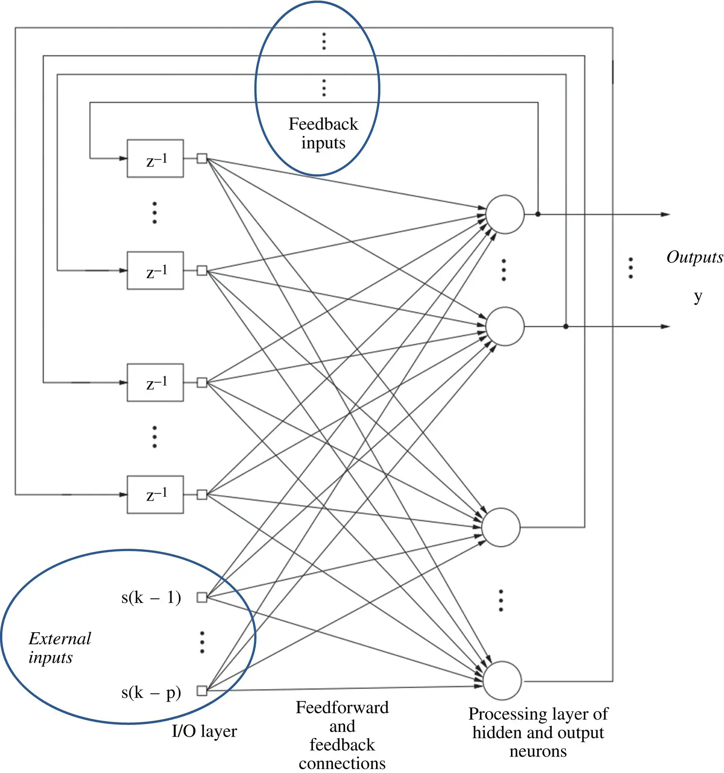
Figure 3.17 A fully connected recurrent neural network (RNN; Williams–Zipser network) The neurons (nodes) are depicted by circles and incorporate the operation Φ (sum of inputs).

Since the external signal vector s does not depend on the elements of W, the error gradient becomes ∂e ( k )/ ∂ω n,l( k ) = − ∂y 1( k )/ ∂ω n,l( k ). Using the chain rule gives

(3.68)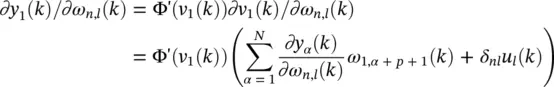

where δ nl= 1 if n = l and 0 otherwise. When the learning rate η is sufficiently small, we have ∂y α( k − 1)/ ∂ω n, l( k ) ≈ ∂y α( k − 1)/ ∂ω n, l( k − 1). By introducing the notation we have recursively for every time step k and all appropriate j , n and l

(3.69)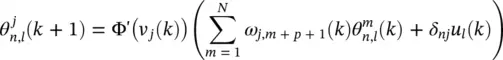

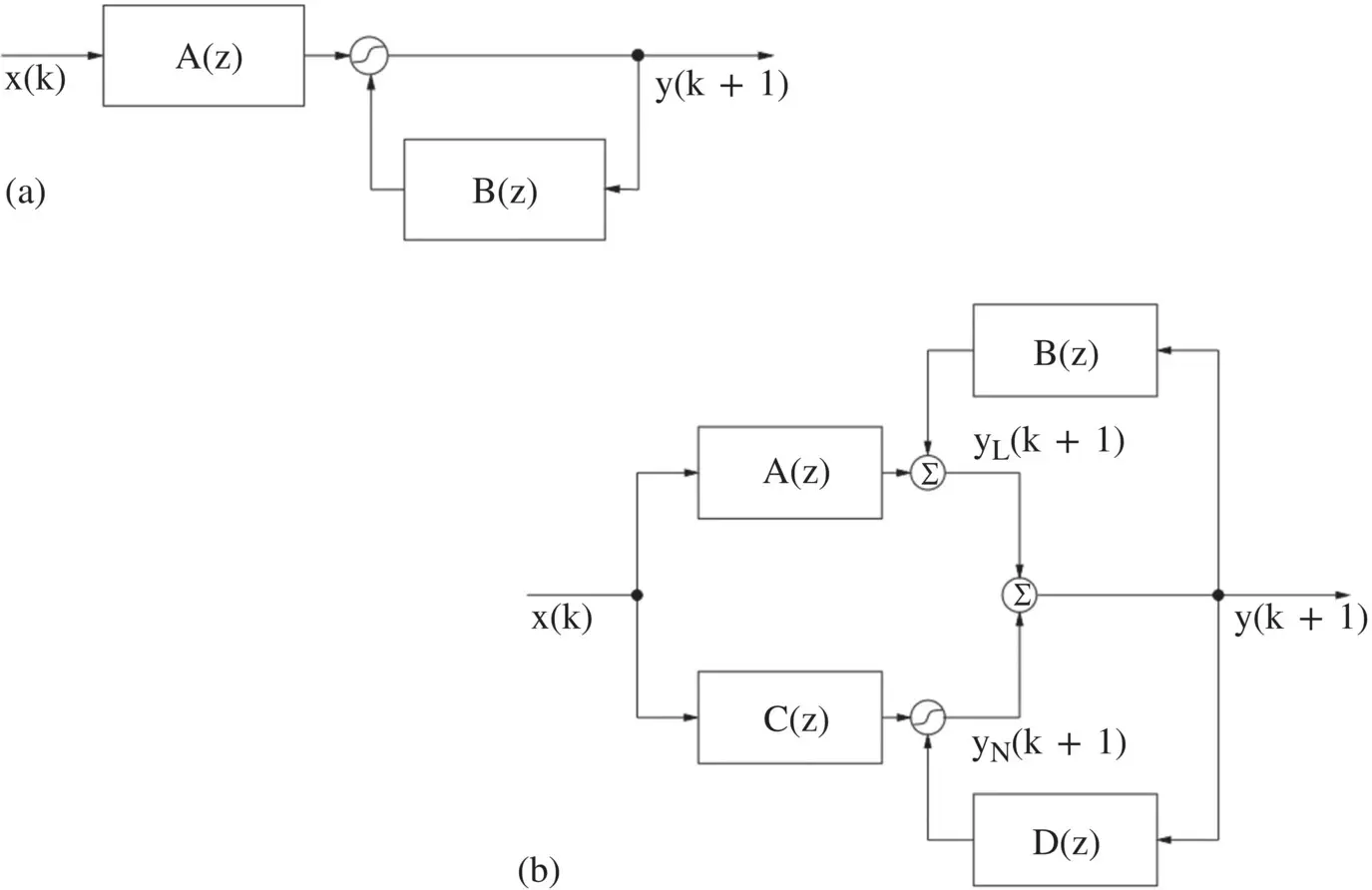
Figure 3.18 Nonlinear IIR filter structures. (a) A recurrent nonlinear neural filter, (b) a recurrent linear/nonlinear neural filter structure.

with the initial conditions . We introduce three new matrices, the N × (N + p + 1) matrix Θ j( k ), the N × (N + p + 1) matrix U j (k) , and the N × N diagonal matrix F(k) , as

(3.70)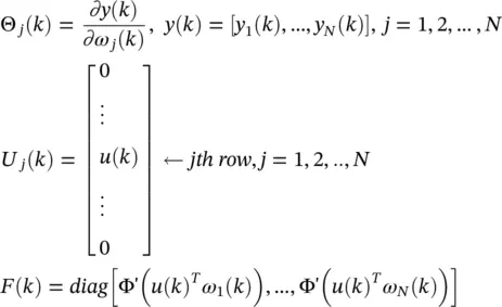

With this notation, the gradient updating equation regarding the recurrent neuron can be symbolically expressed as

(3.71)

where W αdenotes the set of those entries in W that correspond to the feedback connections.

The most popular RNN architectures for sequence learning evolved from long short ‐ term memory ( LSTM ) [8] and bidirectional recurrent neural networks ( BRNNs ) [9] schemes. The former introduces the memory cell, a unit of computation that replaces traditional nodes in the hidden layer of a network. With these memory cells, networks are able to overcome difficulties with training encountered by earlier recurrent networks. The latter introduces an architecture in which information from both the future and the past are used to determine the output at any point in the sequence. This is in contrast to previous networks, in which only past input can affect the output, and has been used successfully for sequence labeling tasks in natural language processing, among others. The two schemes are not mutually exclusive, and have been successfully combined for phoneme classification [10] and handwriting recognition [11]. In this section, we explain the LSTM and BRNN, and we describe the neural Turing machine (NTM), which extends RNNs with an addressable external memory [12].

LSTM scheme: This was introduced primarily in order to overcome the problem of vanishing gradients. This model resembles a standard RNN with a hidden layer, but each ordinary node in the hidden layer is replaced by a memory cell ( Figure 3.19). Each memory cell contains a node with a self‐connected recurrent edge of fixed weight one, ensuring that the gradient can pass across many time steps without vanishing or exploding. To distinguish references to a memory cell and not an ordinary node, we use the subscript c.