Savo G. Glisic - Artificial Intelligence and Quantum Computing for Advanced Wireless Networks

(3.45)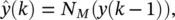

where N Mis an FIR network with total memory length M .

The basic predictor training configuration for the FIR network is shown in Figure 3.9with a known value of y ( k − 1) as the input, and the output as the single‐step estimate of the true series value y ( k ). During training, the squared error is minimized by using the temporal backpropagation algorithm to adapt the network ( y ( k ) acts as the desired response). Training consists of finding a least‐squares solution. In a stochastic framework, the optimal neural network mapping is simply the conditional running mean

Figure 3.9 Network prediction configuration.

(3.46)

where y ( k ) is viewed as a stationary ergodic process‚ and the expectation is taken over the joint distribution of y ( k ) through y ( k − M ). N *represents a closed‐form optimal solution that can only be approximated due to finite training data and constraints in the network topology.

Iterated predictions: Once the network is trained, iterated prediction is achieved by taking the estimate and feeding it back as input to the network:

(3.47)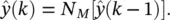

as illustrated in Figure 3.9. Equation (3.47)can be now iterated forward in time to achieve predictions as far into the future as desired. Suppose, for example, that we were given only N points for some time series of interest. We would train the network on those N points. The single‐step estimate , based on known values of the series, would then be fed back to produce the estimate , and continued iterations would yield future predictions.

Linear filters: As already indicated so far in this chapter, linear filters have been exploited for the structures of predictors. In general, there are two families of filters: those without feedback, whose output depends only upon current and past input values; and those with feedback, whose output depends upon both input values and past outputs. Such filters are best described by a constant coefficient difference equation, as

(3.48)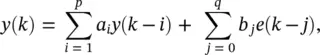

where y ( k ) is the output, e ( k ) is the input, a i, i = 1, 2, … , p , are the AR feedback coefficients and b j, j = 0, 1, … , q , are the moving average (MA) feedforward coefficients. Such a filter is termed an autoregressive moving average (ARMA ( p , q )) filter, where p is the order of the autoregressive, or feedback, part of the structure, and q is the order of the MA, or feedforward, element of the structure. Due to the feedback present within this filter, the impulse response – that is, the values of ( k ), k ≥ 0, when e ( k ) is a discrete time impulse – is infinite in duration, and therefore such a filter is referred to as an infinite impulse response (IIR) filter.

The general form of Eq. (3.48)is simplified by removing the feedback terms as

(3.49)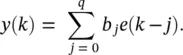

Such a filter is called MA ( q ) and has an FIR that is identical to the parameters b j, j = 0, 1, … , q . In digital signal processing, therefore, such a filter is called an FIR filter. Similarly, Eq. (3.48)is simplified to yield an autoregressive (AR(p)) filter

(3.50)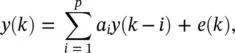

which is also an IIR filter. The filter described by Eq. (3.50)is the basis for modeling the speech generating process. The presence of feedback within the AR( p ) and ARMA ( p , q ) filters implies that selection of the a i, i = 1, 2, … , p , coefficients must be such that the filters are bounded input bounded output ( BIBO ) stable. The most straightforward way to test stability is to exploit the ‐domain representation of the transfer function of the filter represented by (3.48):

(3.51)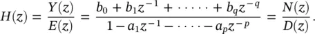

To guarantee stability, the p roots of the denominator polynomial of ( z ), that is, the values of z for which D ( z ) = 0, the poles of the transfer function, must lie within the unit circle in the z ‐plane, ∣ z ∣ < 1.

Nonlinear predictors: If a measurement is assumed to be generated by an ARMA ( p , q ) model, the optimal conditional mean predictor of the discrete time random signal { y ( k )}

(3.52)

is given by

(3.53)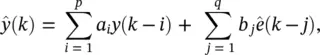

where the residuals ê j = 1, 2, … , q . The feedback present within Eq. (3.53), which is due to the residuals ê ( k − j ), results from the presence of the MA ( q ) part of the model for y ( k ) in Eq. (3.48). No information is available about e ( k ), and therefore it cannot form part of the prediction. On this basis, the simplest form of nonlinear autoregressive moving average (NARMA ( p , q )) model takes the form