Savo G. Glisic - Artificial Intelligence and Quantum Computing for Advanced Wireless Networks
Здесь есть возможность читать онлайн «Savo G. Glisic - Artificial Intelligence and Quantum Computing for Advanced Wireless Networks» — ознакомительный отрывок электронной книги совершенно бесплатно, а после прочтения отрывка купить полную версию. В некоторых случаях можно слушать аудио, скачать через торрент в формате fb2 и присутствует краткое содержание. Жанр: unrecognised, на английском языке. Описание произведения, (предисловие) а так же отзывы посетителей доступны на портале библиотеки ЛибКат.

- Название:Artificial Intelligence and Quantum Computing for Advanced Wireless Networks
- Автор:
- Жанр:
- Год:неизвестен
- ISBN:нет данных
- Рейтинг книги:3 / 5. Голосов: 1
-
Избранное:Добавить в избранное
- Отзывы:
-
Ваша оценка:
Artificial Intelligence and Quantum Computing for Advanced Wireless Networks: краткое содержание, описание и аннотация
Предлагаем к чтению аннотацию, описание, краткое содержание или предисловие (зависит от того, что написал сам автор книги «Artificial Intelligence and Quantum Computing for Advanced Wireless Networks»). Если вы не нашли необходимую информацию о книге — напишите в комментариях, мы постараемся отыскать её.
A practical overview of the implementation of artificial intelligence and quantum computing technology in large-scale communication networks Artificial Intelligence and Quantum Computing for Advanced Wireless Networks
Artificial Intelligence and Quantum Computing for Advanced Wireless Networks
Artificial Intelligence and Quantum Computing for Advanced Wireless Networks — читать онлайн ознакомительный отрывок
Ниже представлен текст книги, разбитый по страницам. Система сохранения места последней прочитанной страницы, позволяет с удобством читать онлайн бесплатно книгу «Artificial Intelligence and Quantum Computing for Advanced Wireless Networks», без необходимости каждый раз заново искать на чём Вы остановились. Поставьте закладку, и сможете в любой момент перейти на страницу, на которой закончили чтение.
Интервал:
Закладка:
(3.54) 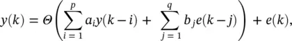
where Θ (·) is an unknown differentiable zero‐memory nonlinear function. Notice e ( k ) is not included within Θ (·) as it is unobservable. The term NARMA ( p , q ) is adopted to define Eq. (3.54), since except for the ( k ), the output of an ARMA ( p , q ) model is simply passed through the zero‐memory nonlinearity Θ (·).
The corresponding NARMA ( p , q ) predictor is given by
(3.55) 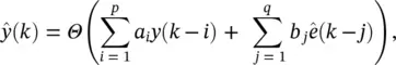
where the residuals ê  j = 1, 2, … , q . Equivalently, the simplest form of nonlinear autoregressive (NAR( p )) model is described by
(3.56) 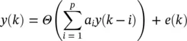
and its associated predictor is
(3.57) 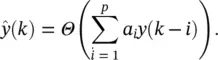
The two predictors are shown together in Figure 3.10, where it is clearly indicated which parts are included in a particular scheme. In other words, feedback is included within the NARMA ( p , q ) predictor, whereas the NAR( p ) predictor is an entirely feedforward structure. In control applications, most generally, NARMA ( p , q ) models also include also external (exogeneous) inputs, ( k − s ), s = 1, 2, … , r , giving
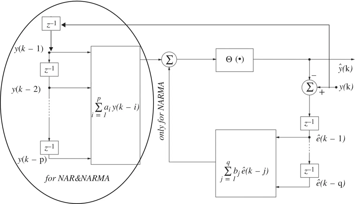
Figure 3.10 Nonlinear AR/ARMA predictors.
(3.58) 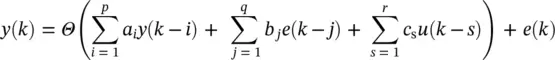
and referred to as a NARMA with exogenous inputs model, NARMAX ( p , q , r ), with associated predictor
(3.59) 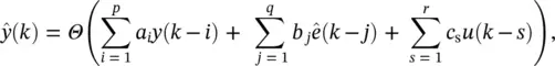
which again exploits feedback.
3.4.2 Feedback Options in Recurrent Neural Networks
Feedbacks in recurrent neural networks: In Figure 3.11, the inputs to the network are drawn from the discrete time signal ( k ). Conceptually, it is straightforward to consider connecting the delayed versions of the output,  , of the network to its input. Such connections, however, introduce feedback into the network, and therefore the stability of such networks must be considered . The provision of feedback, with delay, introduces memory to the network and so is appropriate for prediction. The feedback within recurrent neural networks can be achieved in either a local or global manner. An example of a recurrent neural network is shown in Figure 3.11with connections for both local and global feedback. The local feedback is achieved by the introduction of feedback within the hidden layer, whereas the global feedback is produced by the connection of the network output to the network input. Interneuron connections can also exist in the hidden layer, but they are not shown in Figure 3.11. Although explicit delays are not shown in the feedback connections, they are assumed to be present within the neurons for the network to be realizable. The operation of a recurrent neural network predictor that employs global feedback can now be represented by
(3.60) 
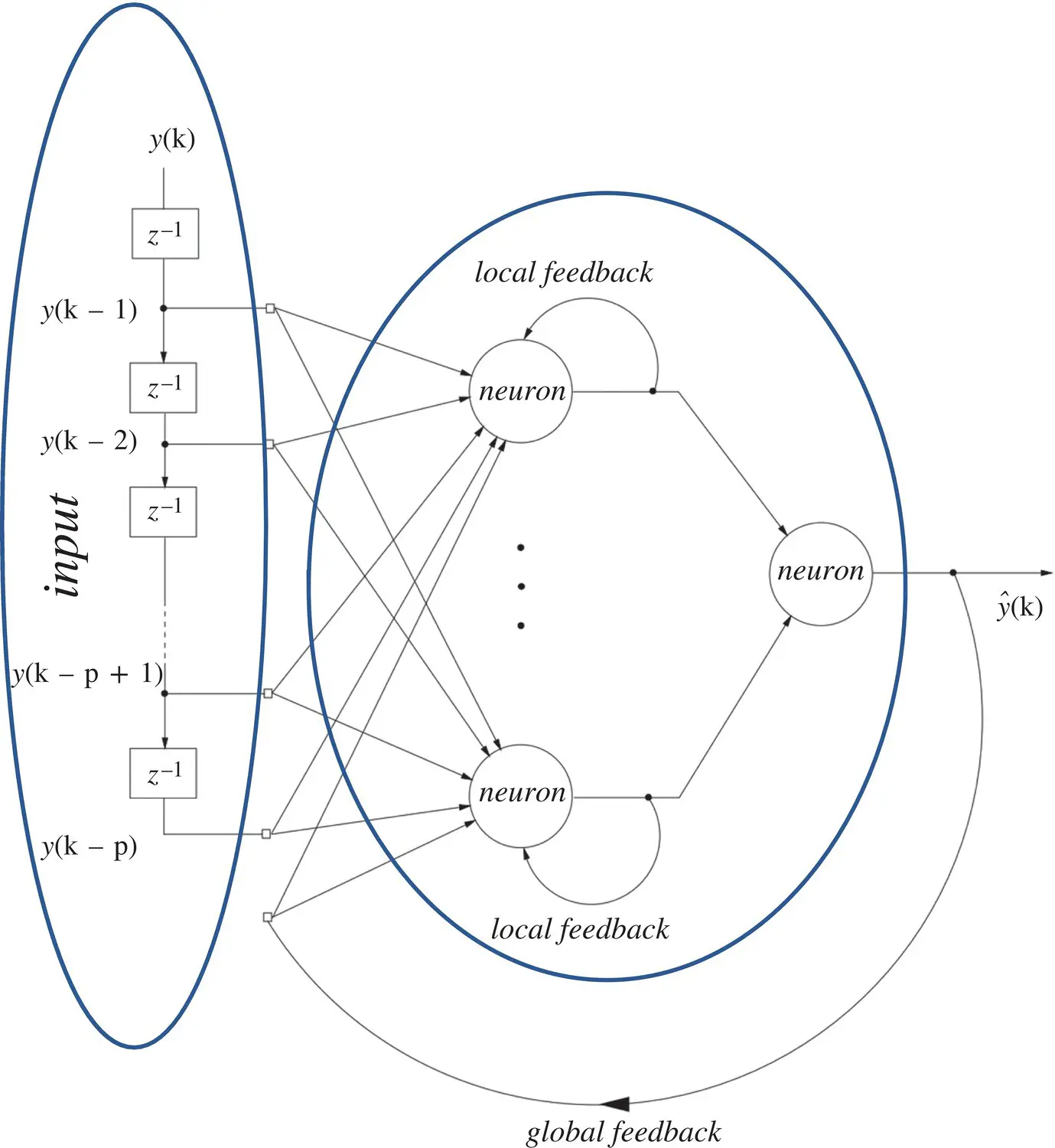
Figure 3.11 Recurrent neural network.
where again Φ (·) represents the nonlinear mapping of the neural network and ê  , j = 1, … , q .
State‐space representation and canonical form: Any feedback network can be cast into a canonical form that consists of a feedforward (static) network (FFSN) (i) whose outputs are the outputs of the neurons that have the desired values, and the values of the state variables, and (ii) whose inputs are the inputs of the network and the values of the state variables, the latter being delayed by one time unit.
The general canonical form of a recurrent neural network is represented in Figure 3.12. If the state is assumed to contain N variables, then a state vector is defined as s ( k ) = [ s 1( k ), s 2( k ), … , s N( k )] T, and a vector of p external inputs is given by y ( k − 1) = [ y ( k − 1), y ( k − 2), … , y ( k − p )] T. The state evolution and output equations of the recurrent network for prediction are given, respectively, by
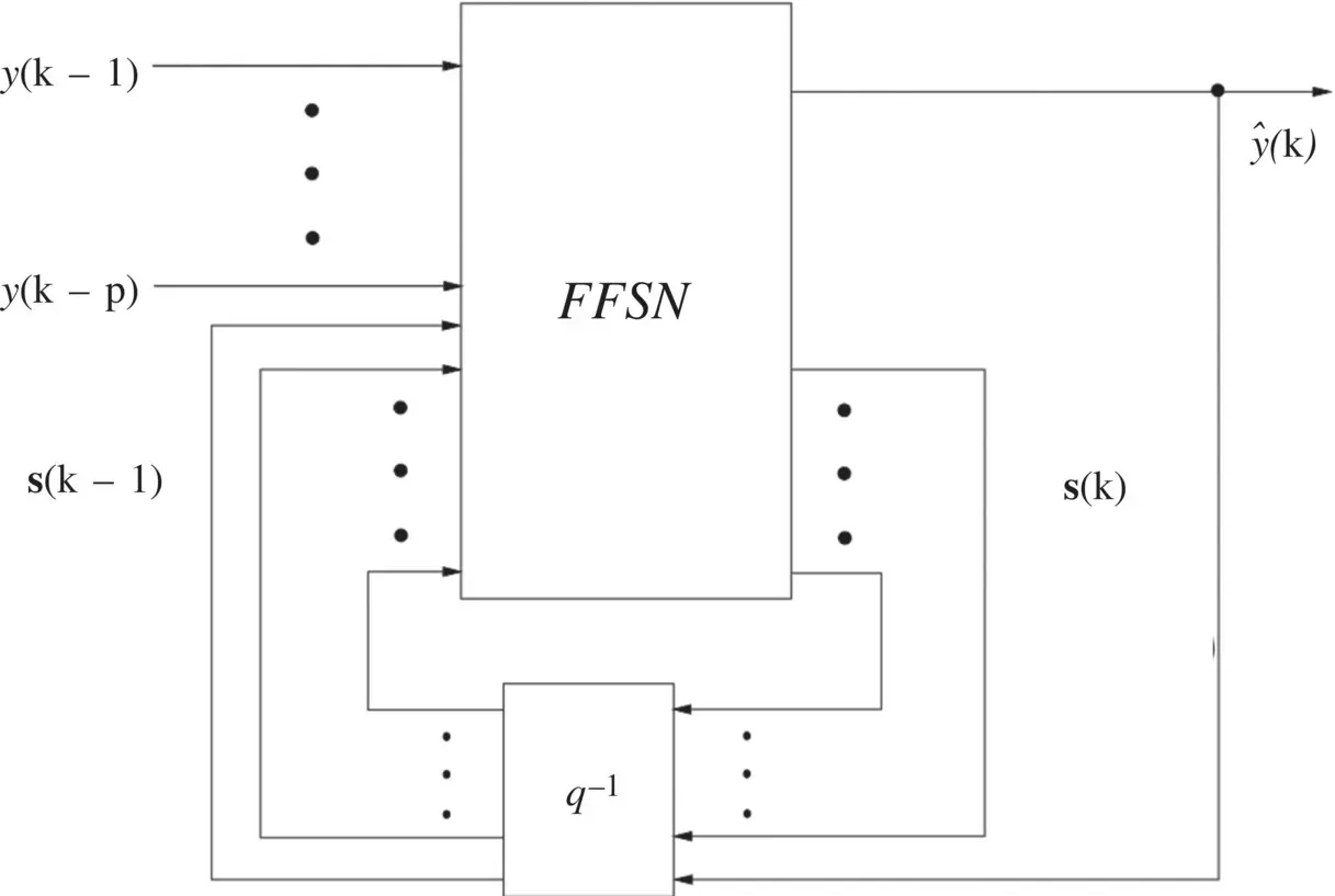
Figure 3.12 Canonical form of a recurrent neural network for prediction.
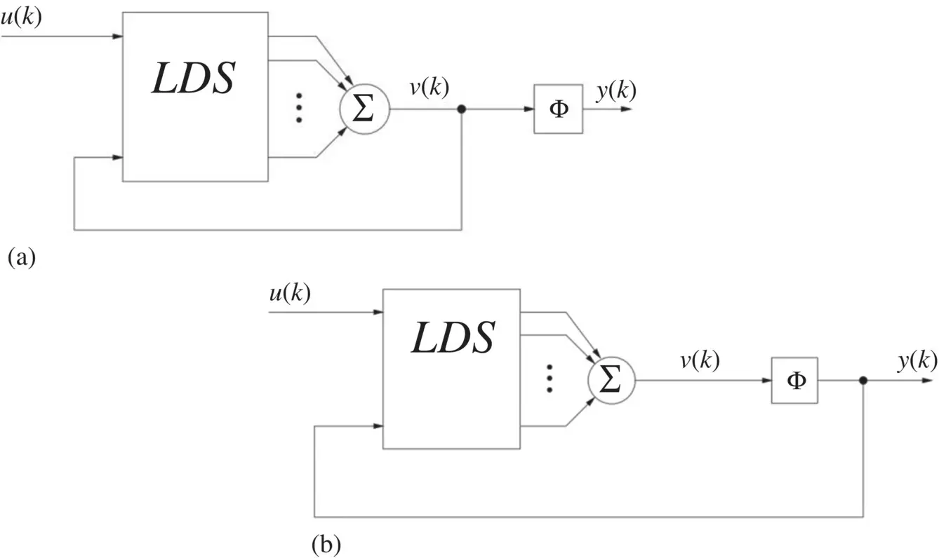
Figure 3.13 Recurrent neural network (RNN) architectures: (a) activation feedback and (b) output feedback.
(3.61) 
(3.62) 
where φ and Ψ represent general classes of nonlinearities.
Recurrent neural network (RNN) architectures: Activation feedback and output feedback are two ways to include recurrent connections in neural networks, as shown in Figure 3.13a and b, respectively.
The output of a neuron shown in Figure 3.13a can be expressed as
(3.63) 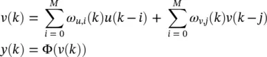
Интервал:
Закладка:
Похожие книги на «Artificial Intelligence and Quantum Computing for Advanced Wireless Networks»
Представляем Вашему вниманию похожие книги на «Artificial Intelligence and Quantum Computing for Advanced Wireless Networks» списком для выбора. Мы отобрали схожую по названию и смыслу литературу в надежде предоставить читателям больше вариантов отыскать новые, интересные, ещё непрочитанные произведения.


Обсуждение, отзывы о книге «Artificial Intelligence and Quantum Computing for Advanced Wireless Networks» и просто собственные мнения читателей. Оставьте ваши комментарии, напишите, что Вы думаете о произведении, его смысле или главных героях. Укажите что конкретно понравилось, а что нет, и почему Вы так считаете.