Savo G. Glisic - Artificial Intelligence and Quantum Computing for Advanced Wireless Networks
Здесь есть возможность читать онлайн «Savo G. Glisic - Artificial Intelligence and Quantum Computing for Advanced Wireless Networks» — ознакомительный отрывок электронной книги совершенно бесплатно, а после прочтения отрывка купить полную версию. В некоторых случаях можно слушать аудио, скачать через торрент в формате fb2 и присутствует краткое содержание. Жанр: unrecognised, на английском языке. Описание произведения, (предисловие) а так же отзывы посетителей доступны на портале библиотеки ЛибКат.

- Название:Artificial Intelligence and Quantum Computing for Advanced Wireless Networks
- Автор:
- Жанр:
- Год:неизвестен
- ISBN:нет данных
- Рейтинг книги:3 / 5. Голосов: 1
-
Избранное:Добавить в избранное
- Отзывы:
-
Ваша оценка:
Artificial Intelligence and Quantum Computing for Advanced Wireless Networks: краткое содержание, описание и аннотация
Предлагаем к чтению аннотацию, описание, краткое содержание или предисловие (зависит от того, что написал сам автор книги «Artificial Intelligence and Quantum Computing for Advanced Wireless Networks»). Если вы не нашли необходимую информацию о книге — напишите в комментариях, мы постараемся отыскать её.
A practical overview of the implementation of artificial intelligence and quantum computing technology in large-scale communication networks Artificial Intelligence and Quantum Computing for Advanced Wireless Networks
Artificial Intelligence and Quantum Computing for Advanced Wireless Networks
Artificial Intelligence and Quantum Computing for Advanced Wireless Networks — читать онлайн ознакомительный отрывок
Ниже представлен текст книги, разбитый по страницам. Система сохранения места последней прочитанной страницы, позволяет с удобством читать онлайн бесплатно книгу «Artificial Intelligence and Quantum Computing for Advanced Wireless Networks», без необходимости каждый раз заново искать на чём Вы остановились. Поставьте закладку, и сможете в любой момент перейти на страницу, на которой закончили чтение.
Интервал:
Закладка:
(3.7) 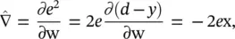
so that Δw = 2 μe x. From this, we have Δ w i= 2 μex i, which is the least mean square (LMS) algorithm.
In a multi‐layer network , we just formally extend this procedure. For this we use the chain rule
(3.8) 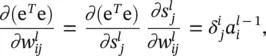
with 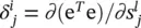 leading to the weight update
 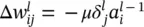 .
.
Parameters δ are derived recursively starting from the output layer:
(3.9) 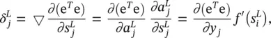
where f ′  is the derivative of the sigmoid function of s . We have also used for the output layer
  . With this, at the output layer, each neuron has an explicit desired response, so we can write
(3.10) 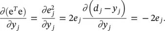
Substituting into Eq. (3.9)yields  .
.
To calculate the δ ′ s , we note that e Te is influenced through  indirectly through all node values
  in the next layer. Referring to the upper part of Figure 3.3, we again employ the chain rule
(3.11) 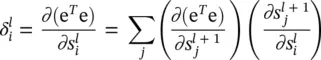
with
(3.12) 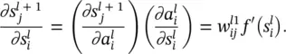
Recalling that  , we get
  In summary, we have
(3.13) 
(3.14) 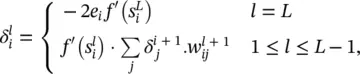
For the bias weight  we note that
  in Eq. (3.13). The above processing is illustrated in Figure 3.4, indicating the symmetry between the forward propagation of neuron activation values and the backward propagation of δ terms.
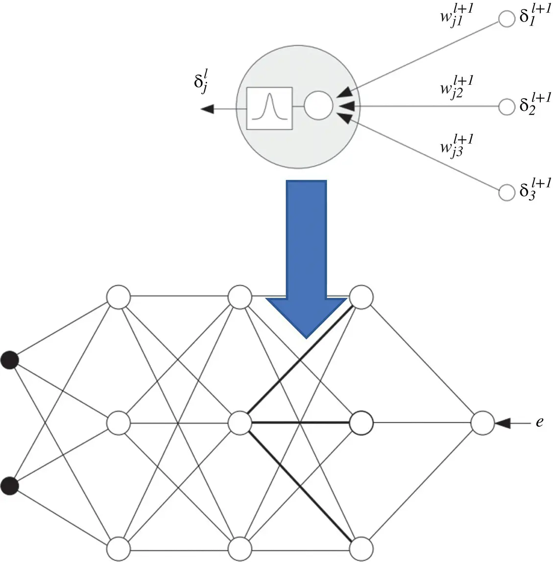
Figure 3.4 Illustration of backpropagation.
3.2 FIR Architecture
3.2.1 Spatial Temporal Representations
Most often in engineering, prior to becoming a member of the observation set, the input signals to the neural network have gone through some form of filtering. This also coincides with the form of potential maintained at the axon hillock region of the neural cell. With this in mind, we may modify Eq. (3.1)as
(3.15) 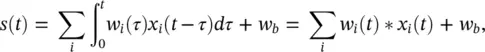
By adding filtering operations, we have included the equally important temporal dimension in the static model. For our purposes, we will now be interested in adapting the filters. To this end, we assume a discrete FIR representation for each filter. This yields
(3.16) 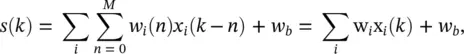
with k being the discrete time index for some sampling rate Δ t , and w i( n ) being the coefficients for the FIR filters. In the following, we will represent the vector w i= [ w i(0), w i(1), … , w i( M )] and the delayed states as x i( k ) = [ x i( k ), x i( k − 1), … , x i( k − M )]. Now, a filter operation is written as the vector dot product w ix i( k ), with time implicitly included in the notation.
The top part of Figure 3.5shows a standard representation of an FIR filter as a tap delay line. Although this filter represents several biological processes, as well as many engineering solutions, for ease of reference to a real neuron network we will refer to an FIR filter as a synaptic filter or simply a synapse . The output of the neuron will be as before y ( k ) = f ( s ( k )) with f ( x ) = tanh ( x ), and we have added only a time index k .
We use the same approach to network modeling as in the previous section. Each link in the network is now created using an FIR filter (see Figure 3.5). The neural network no longer performs a simple static mapping from input to output; internal memory has now been added to simple static mapping from input to output. At the same time, since there are no feedback loops, the overall network is still FIR [2–5]. The notation now becomes 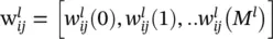 .
.
Интервал:
Закладка:
Похожие книги на «Artificial Intelligence and Quantum Computing for Advanced Wireless Networks»
Представляем Вашему вниманию похожие книги на «Artificial Intelligence and Quantum Computing for Advanced Wireless Networks» списком для выбора. Мы отобрали схожую по названию и смыслу литературу в надежде предоставить читателям больше вариантов отыскать новые, интересные, ещё непрочитанные произведения.


Обсуждение, отзывы о книге «Artificial Intelligence and Quantum Computing for Advanced Wireless Networks» и просто собственные мнения читателей. Оставьте ваши комментарии, напишите, что Вы думаете о произведении, его смысле или главных героях. Укажите что конкретно понравилось, а что нет, и почему Вы так считаете.