Savo G. Glisic - Artificial Intelligence and Quantum Computing for Advanced Wireless Networks

Multi‐layer neural networks: A neural network is built up by incorporating the basic neuron model into different configurations. One example is the Hopfield network, where the output of each neuron can have a connection to the input of all neurons in the network, including a self‐feedback connection. Another option is the multi ‐ layer feedforward network illustrated in Figure 3.2. Here, we have layers of neurons where the output of a neuron in a given layer is input to all the neurons in the next layer. We may also have sparse connections or direct connections that may bypass layers. In these networks, no feedback loops exist within the structure. These network are sometimes referred to as backpropagation networks .

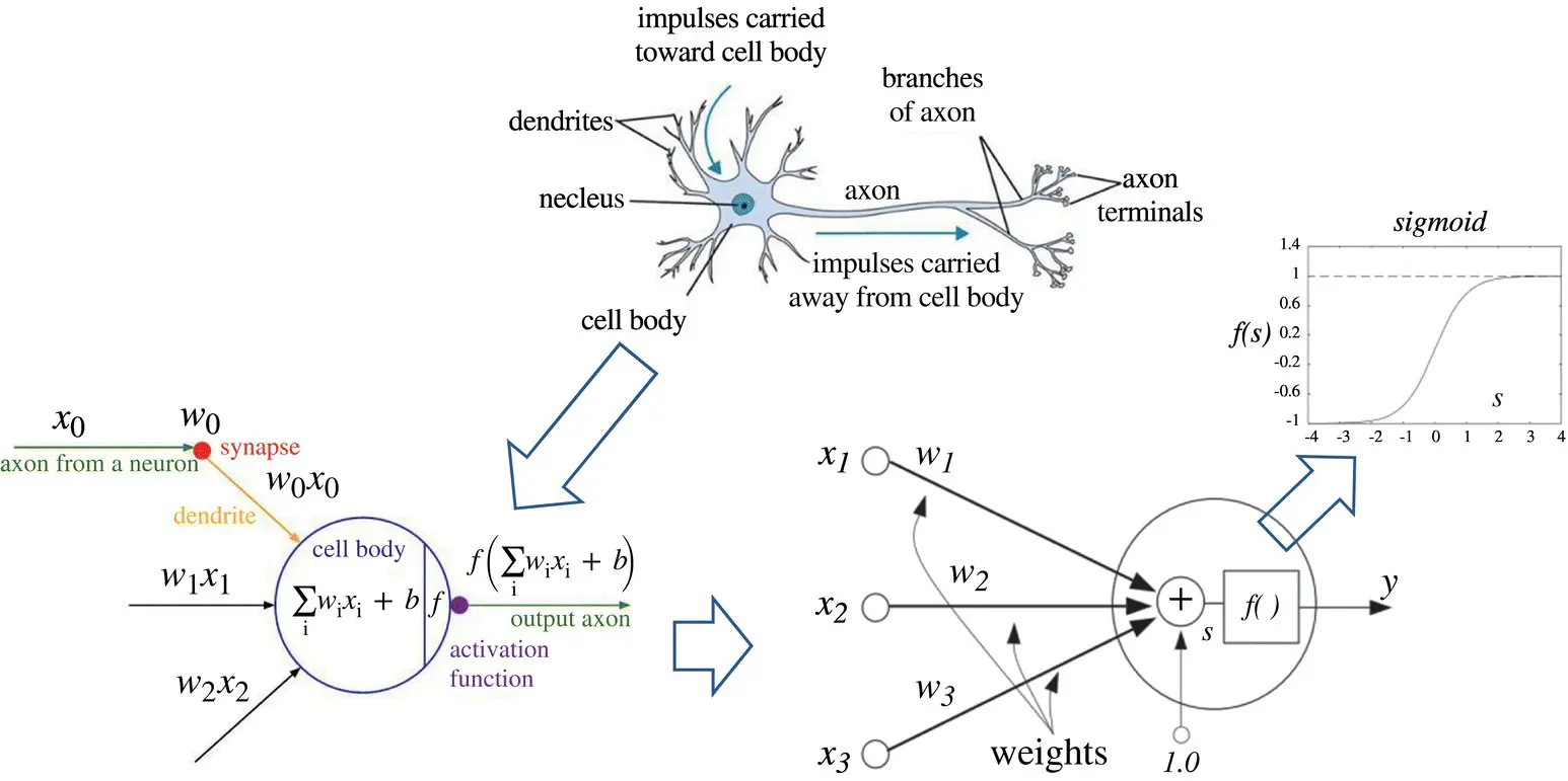
Figure 3.1 From biological to mathematical simplified model of a neuron.

Source: CS231n Convolutional Neural Networks for Visual Recognition [1].

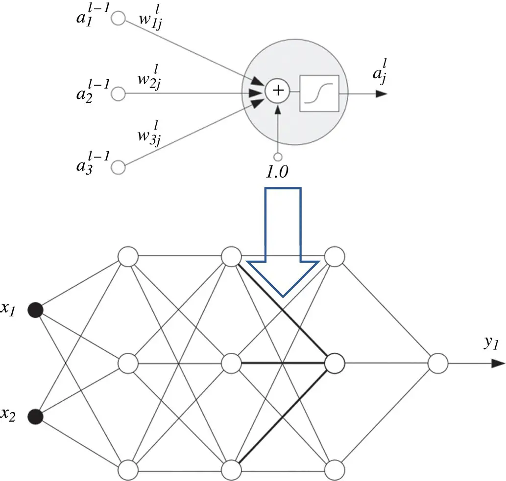
Figure 3.2 Block diagram of feedforward network.

Notation: A single neuron extracted from the l ‐th layer of an L ‐layer network is also depicted in Figure 3.2. Parameters denote the weights on the links between neuron i in the previous layer and neuron j in layer l . The output of the j ‐th neuron in layer l is represented by the variable . The outputs in the last L ‐th layer represent the overall outputs of the network. Here, we use notation y ifor the outputs as . Parameters x i, defined as inputs to the network, may be viewed as a 0‐th layer with notation . These definitions are summarized in Table 3.1.

Table 3.1 Multi‐layer network notation.

	Weight connecting neuron i in layer l − 1 to neuron j in layer l
	Bias weight for neuron j in layer l
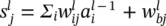	Summing junction for neuron j in layer l
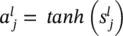	Activation (output) value for neuron j in layer l
	i ‐th external input to network
	i ‐th output to network

Define an input vector x = [ x 0, x 1, x 2, … x N] and output vector y = [ y 0, y 1, y 2, … y M]. The network maps, y = N ( w , x ), the input x to the outputs y using the weights w. Since fixed weights are used, this mapping is static ; there are no internal dynamics. Still, this network is a powerful tool for computation.

It has been shown that with two or more layers and a sufficient number of internal neurons, any uniformly continuous function can be represented with acceptable accuracy. The performance rests on the ways in which this “universal function approximator” is utilized.

The specific mapping with a network is obtained by an appropriate choice of weight values. Optimizing a set of weights is referred to as network training. An example of supervised learning scheme is shown in Figure 3.3. A training set of input vectors associated with the desired output vector, {(x 1, d 1), … (x P, d P)}, is provided. The difference between the desired output and the actual output of the network, for a given input sequence x, is defined as the error

(3.3)

The overall objective function to be minimized over the training set is the given squared error

(3.4)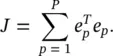

The training should find the set of weights w that minimizes the cost J subject to the constraint of the network topology. We see that training a neural network represent a standard optimization problem.

A stochastic gradient descent (SGD) algorithm is an option as an optimization method. For each sample from the training set, the weights are adapted as

(3.5)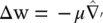

where is the error gradient for the current input pattern, and μ is the learning rate.

Backpropagation: This is a standard way to find in Eq. (3.5). Here we provide a formal derivation.

Single neuron case – Consider first a single linear neuron, which we may describe compactly as

(3.6)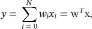

where w = [ w 0, w 1, … w N] and x = [1, x 1, … x N]. In this simple setup

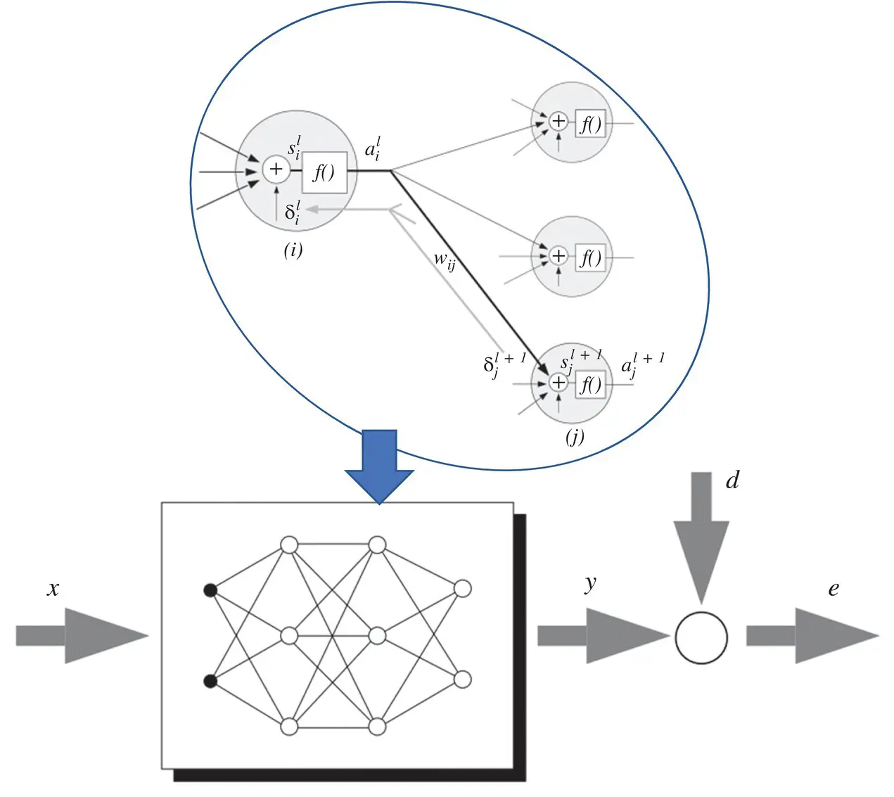
Figure 3.3 Schematic representation of supervised learning.