Savo G. Glisic - Artificial Intelligence and Quantum Computing for Advanced Wireless Networks

11 11 Kohavi, R. and Quinlan, J.R. (2002, ch. 16.1.3). Decision‐tree discovery. In: Handbook of Data Mining and Knowledge Discovery (eds. W. Klosgen and J.M. Zytkow), 267–276. London, U.K.: Oxford University Press.

12 12 Hastie, T. Trees, Bagging, Random Forests and Boosting. Stanford University lecture notes.

13 13 Hancock, T.R., Jiang, T., Li, M., and Tromp, J. (1996). Lower bounds on learning decision lists and trees. Inf. Comput. 126 (2): 114–122.

14 14 Hyafil, L. and Rivest, R.L. (1976). Constructing optimal binary decision trees is NP‐complete. Inf. Process. Lett. 5 (1): 15–17.

15 15 Zantema, H. and Bodlaender, H.L. (2000). Finding small equivalent decision trees is hard. Int. J. Found. Comput. Sci. 11 (2): 343–354.

16 16 Naumov, G.E. (1991). NP‐completeness of problems of construction of optimal decision trees. Sov. Phys. Dokl. 36 (4): 270–271.

17 17 Bratko, I. and Bohanec, M. (1994). Trading accuracy for simplicity in decision trees. Mach. Learn. 15: 223–250.

18 18 Almuallim, H. (1996). An efficient algorithm for optimal pruning of decision trees. Artif. Intell. 83 (2): 347–362.

19 19 Rissanen, J. (1989). Stochastic Complexity and Statistical Inquiry. Singapore: World Scientific.

20 20 Quinlan, J.R. and Rivest, R.L. (1989). Inferring decision trees using the minimum description length principle. Inf. Comput. 80: 227–248.

21 21 Mehta, R.L., Rissanen, J., and Agrawal, R. (1995). Proceedings of the 1st International Conference on Knowledge Discovery and Data Mining, pp. 216–221.

22 22 Dash, M. and Liu, H. (1997). Feature selection for classification. Intell. Data Anal. 1: 131–156.

23 23 Guyon, I. and Eliseeff, A. (2003). An introduction to variable and feature selection. J. Mach. Learn. Res. 3: 1157–1182.

24 24 Saeys, Y., Inza, I., and Larrañaga, P. (2007). A review of feature selection techniques in bioinformatics. Bioinformatics 23: 2507–2517.

25 25 Rioul, O. and Vetterli, M. (1991). Wavelets and signal processing. IEEE Signal Process. Mag. 8: 14–38.

26 26 Graps, A. (1995). An introduction to wavelets. IEEE Comput. Sci. Eng. 2: 50–61.

27 27 Huang, H.E., Shen, Z., Long, S.R. et al. (1998). The empirical mode decomposition and the Hilbert spectrum for nonlinear and non‐stationary time series analysis. Proc. R. Soc. Lond. A 454: 903–995.

28 28 Rilling, G.; Flandrin, P. & Goncalves, P. On empirical mode decomposition and its algorithms Proc. IEEE‐EURASIP Workshop on Nonlinear Signal and Image Processing, 2003

29 29 Fisher, R.A. (1936). The use of multiple measurements in taxonomic problems. Ann. Eugen. 7: 179–188.

30 30 Fodor, I.K. (2002). A Survey of Dimension Reduction Techniques. Lawrence Livermore National Laboratory.

31 31 Bian, W. and Tao, D. (2011). Max‐min distance analysis by using sequential SDP relaxation for dimension reduction. IEEE Trans. Pattern Anal. Mach. Intell. 33: 1037–1050.

32 32 Cai, H., Mikolajczyk, K., and Matas, J. (2011). Learning linear discriminant projections for dimensionality reduction of image descriptors. IEEE Trans. Pattern Anal. Mach. Intell. 33: 338–352.

33 33 Kim, M. and Pavlovic, V. (2011). Central subspace dimensionality reduction using covariance operators. IEEE Trans. Pattern Anal. Mach. Intell. 33: 657–670.

34 34 Lin, Y.Y., Liu, T.L., and Fuh, C.S. (2011). Multiple kernel learning for dimensionality reduction. IEEE Trans. Pattern Anal. Mach. Intell. 33: 1147–1160.

35 35 Batmanghelich, N.K., Taskar, B., and Davatzikos, C. (2012). Generative‐discriminative basis learning for medical imaging. IEEE Trans. Med. Imaging 31: 51–69.

36 36 Baraniuk, R.G., Cevher, V., and Wakin, M.B. (2012). Low‐dimensional models for dimensionality reduction and signal recovery: a geometric perspective. Proc. IEEE 98: 959–971.

37 37 Gray, R.M. (1984). Vector quantization IEEE acoustics. Speech Signal Process. Mag. 1: 4–29.

38 38 Gersho, A. and Gray, R.M. (1992). Vector quantization and signal compression. Kluwer Academic Publishers.

39 39 Pearson, K. (1901). On lines and planes of closest fit to systems of points in space. Philos. Mag. 2: 559–572.

40 40 Wold, S., Esbensen, K., and Geladi, P. (1987). Principal component analysis. Chemom. Intel. Lab. Syst. 2: 37–35.

41 41 Dunteman, G.H. (1989). Principal Component Analysis. Sage Publications.

42 42 Jollife, I. T. Principal Component Analysis Wiley, 2002

43 43 Hÿvarinen, A., Karhunen, J., and Oja, E. (2001). Independent Component Analysis. Wiley.

44 44 He, R., Hu, B.‐G., Zheng, W.‐S., and Kong, X.‐W. (2011). Robust principal component analysis based on maximum correntropy criterion. IEEE Trans. Image Process. 20: 1485–1494.

45 45 Li, X.L., Adali, T., and Anderson, M. (2011). Noncircular principal component analysis and its application to model selection. IEEE Trans. Signal Process. 59: 4516–4528.

46 46 Sorzano, C.O.S., Vargas, J., and Pascual‐Montano, A. A survey of dimensionality reduction techniques. https://arxiv.org/ftp/arxiv/papers/1403/1403.2877.pdf

47 47 Jenssen, R. (2010). Kernel entropy component analysis. IEEE Trans. Pattern Anal. Mach. Intell. 32: 847–860.

48 48 https://medium.com/machine‐learning‐101/chapter‐2‐svm‐support‐vector‐machine‐theory‐f0812effc72

49 49 https://cgl.ethz.ch/teaching/former/vc_master_06/Downloads/viscomp‐svm‐clustering_6.pdf

50 50 https://people.duke.edu/~rnau/regintro.htm

51 51 https://discuss.analyticsvidhya.com/t/what‐does‐min‐samples‐split‐means‐in‐decision‐tree/6233

52 52 https://medium.com/@mohtedibf/indepth‐parameter‐tuning‐for‐decision‐tree‐6753118a03c3

53 53 https://gist.github.com/PulkitS01/97c9920b1c913ba5e7e101d0e9030b0e

A biological [1] and mathematical model of a neuron can be represented as shown in Figure 3.1with the output of the neuron modeled as

(3.1)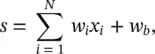

(3.2)

where x iare the inputs to the neuron, w iare the synaptic weights, and w bmodels a bias . In general, f represents the nonlinear activation function . Early models used a sign function for the activation. In this case, the output y would be +1 or −1 depending on whether the total input at the node s exceeds 0 or not. Nowadays, a sigmoid function is used rather than a hard threshold. One should immediately notice the similarity of Eqs. (3.1)and (3.2)with Eqs. (2.1)and (2.2)defining the operation of a linear predictor. This should suggest that in this chapter we will take the problem of parameter estimation to the next level. The sigmoid, shown in Figure 3.1, is a differentiable squashing function usually evaluated as y = tanh ( s ). This engineering model is an oversimplified approximation to the biological model. It neglects temporal relations. This is because the goals of the engineer differ from that of the neurobiologist. The former must use the models feasible for practical implementation. The computational abilities of an isolated neuron are extremely limited.

For electrical engineers, the most popular applications of single neurons are in adaptive finite impulse response (FIR) filters. Here, 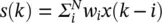, where k represents a discrete time index. Usually, a linear activation function is used. In electrical engineering, adaptive filters are used in signal processing with practical applications like adaptive equalization, and active noise cancelation.