Savo G. Glisic - Artificial Intelligence and Quantum Computing for Advanced Wireless Networks

Vector quantization and mixture models : Probably the simplest way of reducing dimensionality is by assigning a class {among a total of K classes) to each one of the observations x n. This can be seen as an extreme case of dimensionality reduction in which we go from M dimensions to 1 (the discrete class label χ ). Each class, χ , has a representative which is the average of all the observations assigned to that class. If a vector x nhas been assigned to the χ n‐th class, then its approximation after the dimensionality reduction is simply , (see Figure 2.19).

The goal is thus to find the representatives , and class assignment u χ(x)( u χ(x) is equal to 1 if the observation x is assigned to the χ ‐th class, and is 0 otherwise) such that 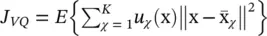is minimized. This problem is known as vector quantization or k‐means , already briefly introduced in Section 2.1. The optimization of this goal function is a combinatorial problem, although there are heuristics to cut down its cost [37, 38]. An alternative formulation of the k‐means objective function is 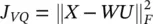subject to U t U = I and u ij∈ {0, 1} {i.e. that each input vector is assigned to one and only one class). 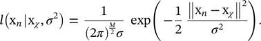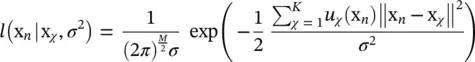In this expression, W is a M × m matrix with all representatives as column vectors, U is an m × N matrix whose ij ‐th entry is 1 if the j ‐th input vector is assigned to the i ‐th class, and denotes the Frobenius norm of a matrix. This intuitive goal function can be put in a probabilistic framework. Let us assume we have a generative model of how the data is produced. Let us assume that the observed data are noisy versions of K vectors x χwhich are equally likely a priori. Let us assume that the observation noise is normally distributed with a spherical covariance matrix = σ 2 I . The likelihood of observing x nhaving produced x χis

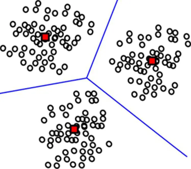
Figure 2.19 Black circles represent the input data, x n; gray squares represent class representatives,

With our previous definition of u χ(x), we can express it as

The log likelihood of observing the whole dataset x n{ n = 1, 2, …, N ) after removing all constants is We thus see that the goal function of vector quantization J VQproduces the maximum likelihood estimates of the underlying x lvectors.

Under this generative model, the probability density function of the observations is the convolution of a Gaussian function and a set of delta functions located at the x χvectors, that is, a set of Gaussians located at the x χvectors. The vector quantization then is an attempt to find the centers of the Gaussians forming the probability density function of the input data. This idea has been further pursued by Mixture Models , which are a generalization of vector quantization in which, instead of looking only for the means of the Gaussians associated with each class, we also allow each class to have a different covariance matrix ∑ χand different a priori probability π χ. The algorithm looks for estimates of all these parameters by Expectation–Maximization , and at the end produces for each input observation x n, the label χ of the Gaussian that has the maximum likelihood of having generated that observation.

This concept can be extend and, instead of making a hard class assignment, a fuzzy class assignment can be used by allowing 0 ≤ u χ(x) ≤ 1 and requiring 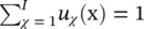for all x. This is another vector quantization algorithm called fuzzy k ‐means . The k‐means algorithm is based on a quadratic objective function, which is known to be strongly affected by outliers. This drawback can be alleviated by taking the l 1norm of the approximation errors and modifying the problem to J K‐medians= subject to U t U = I and u ij∈ {0, 1}. A different approach can be used to find data representatives less affected by outliers, which we may call robust vector quantization, 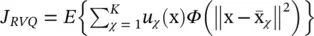, where Φ ( x ) is a function less sensitive to outliers than Φ ( x ) = x , for instance, Φ ( x ) = x αwith α about 0.5.

Principal component analysis (PCA): Introduced in Section 2.1, is by far one of the most popular algorithms for dimensionality reduction [39–42]. Given a set of observations x, with dimension M (they lie in ℝ M), PCA is the standard technique for finding the single best (in the sense of least‐square error) subspace of a given dimension, m . Without loss of generality, we may assume the data is zero‐mean and the subspace to fit is a linear subspace (passing through the origin).

This algorithm is based on the search for orthogonal directions explaining as much variance of the data as possible. In terms of dimensionality reduction, it can be formulated [43] as the problem of finding the m orthonormal directions w iminimizing the representation error 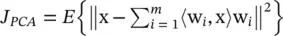. In this objective function, the reduced vectors are the projections χ= (〈w 1, x〉, …, 〈w m, x〉) tThis can be much more compactly written as χ= W tx, where W is a M × m matrix whose columns are the orthonormal directions w i{or equivalently W t W = I ). The approximation to the original vectors is given by 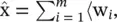x〉w i, or equivalently, W χ.