Savo G. Glisic - Artificial Intelligence and Quantum Computing for Advanced Wireless Networks

Terminology: In a typical supervised learning, a training set of labeled examples is given, and the goal is to form a description that can be used to predict previously unseen examples. Most frequently, the training sets are described as a bag instance of a certain bag schema . The bag schema provides the description of the attributes and their domains. Formally, bag schema is denoted as R ( A ∪ y ), where A denotes the set of n attributes A = { a 1, … a i, … a n}, and y represents the class variable or the target attribute.

Attributes can be nominal or numeric. When the attribute a iis nominal, it is useful to denote by its domain values, where ∣ dom( a i)∣ stands for its finite cardinality. In a similar way, dom( y ) = { c 1, …, c ∣ dom(y)∣} represents the domain of the target attribute. Numeric attributes have infinite cardinalities. The set of all possible examples is called the instance space, which is defined as the Cartesian product of all the input attributes domains: X = dom( a 1) × dom( a 2) × … × dom( a n). The universal instance space (or the labeled instance space) U is defined as the Cartesian product of all input attribute domains and the target attribute domain, that is, U = X × dom( y ). The training set is a bag instance consisting of a set of m tuples (also known as records ). Each tuple is described by a vector of attribute values in accordance with the definition of the bag schema. Formally, the training set is denoted as

Usually, it is assumed that the training set tuples are generated randomly and independently according to some fixed and unknown joint probability distribution D over U . Note that this is a generalization of the deterministic case when a supervisor classifies a tuple using a function y = f ( x ). Here‚ we use the common notation of bag algebra to present the projection ( π ) and selection ( σ ) of tuples.

The ML community, which is target audience of this book, has introduced the problem of concept learning . To learn a concept is to infer its general definition from a set of examples. This definition may be either explicitly formulated or left implicit, but either way it assigns each possible example to the concept or not. Thus, a concept can be formally regarded as a function from the set of all possible examples to the Boolean set {true, false}.

On the other hand, the data mining community prefers to deal with a straightforward extension of the concept learning , known as the classi fi cation problem . In this case, we search for a function that maps the set of all possible examples into a predefined set of class labels and is not limited to the Boolean set.

An inducer is an entity that obtains a training set and forms a classifier that represents the generalized relationship between the input attributes and the target attribute.

The notation I represents an inducer and I ( S ) represents a classifier that was induced by performing I on a training set S . Most frequently, the goal of the classifier’s inducers is formally defined as follows: Given a training set S with input attributes set A = { a 1, a 2, … a n} and a target attribute y from a unknown fi xed distribution D over the labeled instance space , the goal is to induce an optimal classi fi er with minimum generalization error .

Generalization error is defined as the misclassification rate over the distribution D . In case of the nominal attributes, it can be expressed as

(2.11)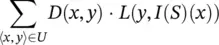

where L ( y , I ( S )( x ) is the loss function defined as L ( y , I ( S )( x )) = 0, if y = I ( S )( x ) and 1, if y ≠ I ( S )( x ). In the case of numeric attributes, the sum operator is replaced with the appropriate integral operator.

Tree representation: The initial examples of tree representation including the pertaining terminology are given in Figures 2.3and 2.4.

The example in Figure 2.16describes a decision tree that reasons whether or not a potential customer will respond to a direct mailing.

Decision tree induction is closely related to rule induction. Each path from the root of a decision tree to one of its leaves can be transformed into a rule simply by conjoining the tests along the path to form the antecedent part, and taking the leaf’s class prediction as the class value. For example, one of the paths in Figure 2.16can be transformed into the rule: “If customer age <30, and the gender of the customer is “male,” then the customer will respond to the mail.”

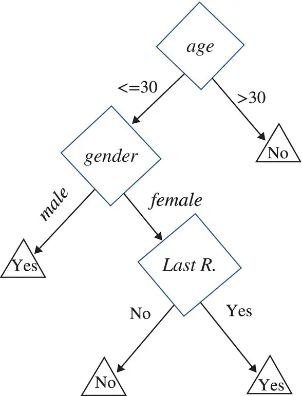
Figure 2.16 Decision tree presenting response to direct mailing.

The goal was to predict whether an email message is spam (junk email) or good.

Input features: Relative frequencies in a message of 57 of the most commonly occurring words and punctuation marks in all the training email messages.

For this problem, not all errors are equal; we want to avoid filtering out good email, while letting spam get through is not desirable but less serious in its consequences.

The spam is coded as 1 and email as 0.

A system like this would be trained for each user separately (e.g. their word lists would be different).

Forty‐eight quantitative predictors – the percentage of words in the email that match a given word. Examples include business, address, Internet, free, and George. The idea was that these could be customized for individual users.

Six quantitative predictors – the percentage of characters in the email that match a given character. The characters are ch;, ch(, ch[, ch!, ch$, and ch#.

The average length of uninterrupted sequences of capital letters: CAPAVE.

The length of the longest uninterrupted sequence of capital letters: CAPMAX.

The sum of the length of uninterrupted sequences of capital letters: CAPTOT.

A test set of size 1536 was randomly chosen, leaving 3065 observations in the training set.

A full tree was grown on the training set, with splitting continuing until a minimum bucket size of 5 was reached.

Algorithmic framework: Decision tree inducers are algorithms that automatically construct a decision tree from a given dataset. Typically, the goal is to find the optimal decision tree by minimizing the generalization error. However, other target functions can be also defined, for instance, minimizing the number of nodes or minimizing the average depth. Induction of an optimal decision tree from a given dataset is a hard task resulting in an NP hard problem [13–16], which is feasible only in small problems. Consequently, heuristic methods are required for solving the problem. Roughly speaking, these methods can be divided into two groups: top‐down and bottom‐up, with a clear preference in the literature to the first group. Figure 2.18presents a typical algorithmic framework for top‐down decision tree induction [8].