Savo G. Glisic - Artificial Intelligence and Quantum Computing for Advanced Wireless Networks
Здесь есть возможность читать онлайн «Savo G. Glisic - Artificial Intelligence and Quantum Computing for Advanced Wireless Networks» — ознакомительный отрывок электронной книги совершенно бесплатно, а после прочтения отрывка купить полную версию. В некоторых случаях можно слушать аудио, скачать через торрент в формате fb2 и присутствует краткое содержание. Жанр: unrecognised, на английском языке. Описание произведения, (предисловие) а так же отзывы посетителей доступны на портале библиотеки ЛибКат.

- Название:Artificial Intelligence and Quantum Computing for Advanced Wireless Networks
- Автор:
- Жанр:
- Год:неизвестен
- ISBN:нет данных
- Рейтинг книги:3 / 5. Голосов: 1
-
Избранное:Добавить в избранное
- Отзывы:
-
Ваша оценка:
Artificial Intelligence and Quantum Computing for Advanced Wireless Networks: краткое содержание, описание и аннотация
Предлагаем к чтению аннотацию, описание, краткое содержание или предисловие (зависит от того, что написал сам автор книги «Artificial Intelligence and Quantum Computing for Advanced Wireless Networks»). Если вы не нашли необходимую информацию о книге — напишите в комментариях, мы постараемся отыскать её.
A practical overview of the implementation of artificial intelligence and quantum computing technology in large-scale communication networks Artificial Intelligence and Quantum Computing for Advanced Wireless Networks
Artificial Intelligence and Quantum Computing for Advanced Wireless Networks
Artificial Intelligence and Quantum Computing for Advanced Wireless Networks — читать онлайн ознакомительный отрывок
Ниже представлен текст книги, разбитый по страницам. Система сохранения места последней прочитанной страницы, позволяет с удобством читать онлайн бесплатно книгу «Artificial Intelligence and Quantum Computing for Advanced Wireless Networks», без необходимости каждый раз заново искать на чём Вы остановились. Поставьте закладку, и сможете в любой момент перейти на страницу, на которой закончили чтение.
Интервал:
Закладка:
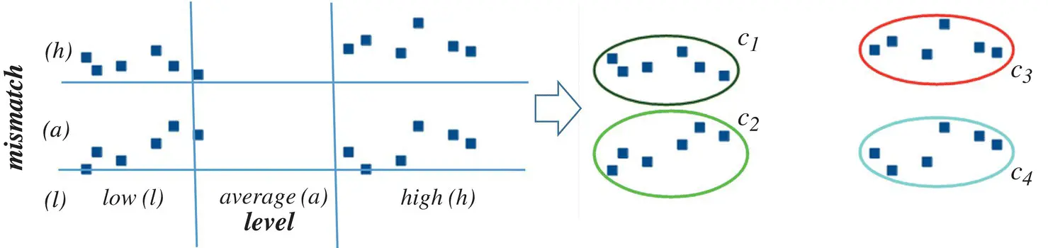
Figure 2.11 Example of clustering.
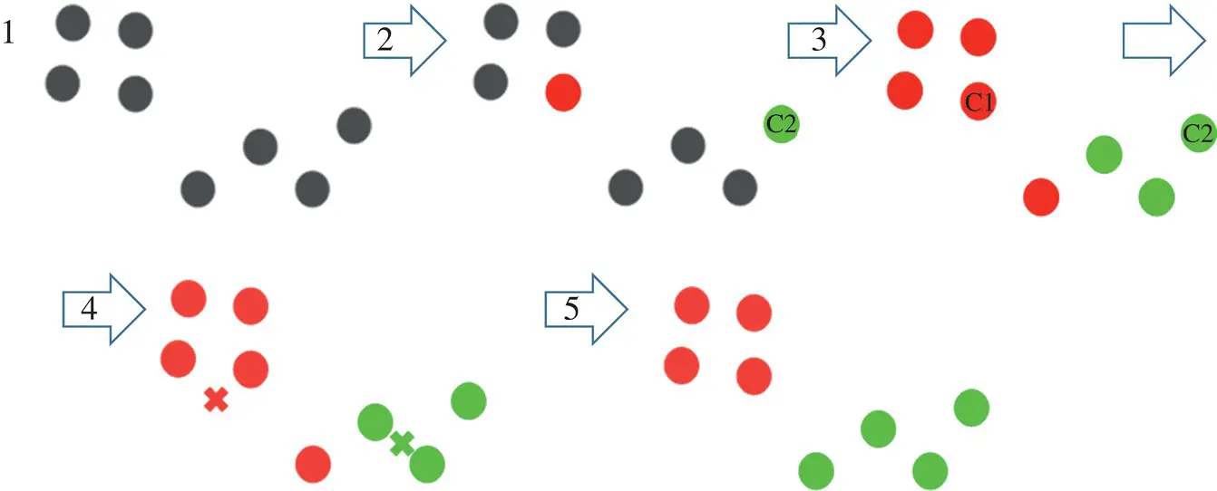
Figure 2.12 k‐Means algorithm.
In k‐means , each cluster is associated with a centroid. The main objective of the k‐means algorithm is to minimize the sum of distances between the points and their respective cluster centroid.
As an example, in Figure 2.12we have eight points, and we want to apply k‐means to create clusters for these points. Here is how we can do it:
1 Choose the number of clusters k.
2 Select k random points from the data as centroids.
3 Assign all the points to the closest cluster centroid.
4 Recompute the centroids of newly formed clusters.
5 Repeat steps 3 and 4.
There are essentially three stopping criteria that can be adopted to stop the k‐means algorithm:
1 Centroids of newly formed clusters do not change.
2 Points remain in the same cluster.
3 The maximum number of iterations is reached.
Meaning three means (k = 3) clustering on 2D dataset using [3] is shown in Figure 2.13.
2.1.9 Dimensionality Reduction
During the last decade, technology has advanced in tremendous ways, and analytics and statistics have played major roles. These techniques fetch an enormous number of datasets that is usually composed of many variables. For instance, the real‐world datasets for image processing, Internet search engines, text analysis, and so on, usually have a higher dimensionality, and to handle such dimensionality, it needs to be reduced but with the requirement that specific information should remain unchanged.
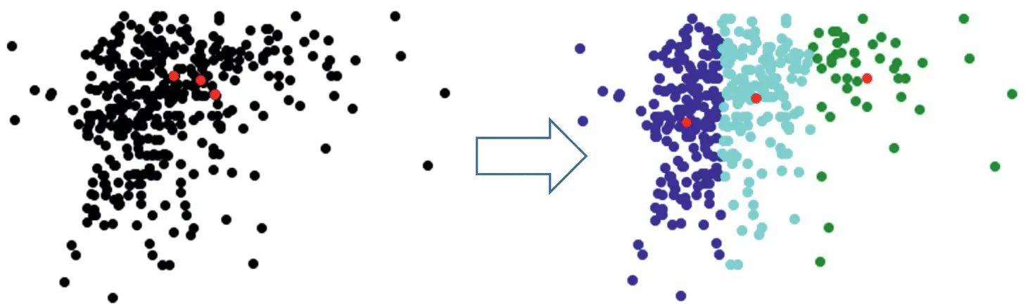
Figure 2.13 k = 3 means clustering on 2D dataset.
Source: Based on PulkitS01 [3], K‐Means implementation, GitHub, Inc. Available at [53], https://gist.github.com/PulkitS01/97c9920b1c913ba5e7e101d0e9030b0e.
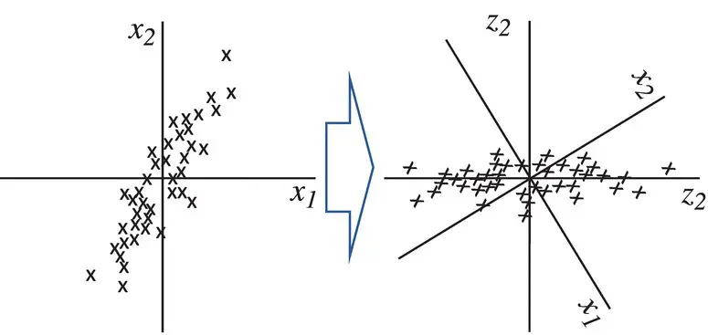
Figure 2.14 Concept of data projection.
Dimensionality reduction [32–34] is a method of converting high‐dimensional variables into lower‐dimensional variables without changing the specific information of the variables. This is often used as a preprocessing step in classification methods or other tasks.
Linear dimensionality reduction linearly projects n ‐dimensional data onto a k ‐dimensional space, k < n, often k < < n ( Figure 2.14).
Design Example 2.2
Principal component analysis (PCA)
The algorithm successively generates principal components (PC): The first PC is the projection direction that maximizes the variance of the projected data. The second PC is the projection direction that is orthogonal to the first PC and maximizes the variance of the projected data. Repeat until k‐orthogonal lines are obtained ( Figure 2.15).
The projected position of a point on these lines gives the coordinates in k ‐dimensional reduced space.
Steps in PCA: (i) Compute covariance matrix ∑ of the dataset S , (ii) calculate the eigenvalues and eigenvectors of ∑ . The eigenvector with the largest eigenvalue λ 1is the first PC. The eigenvector with the k th largest eigenvalue λ kis the k th PC. λ k/ ∑ i λ i= proportion of variance captured by the k th PC.
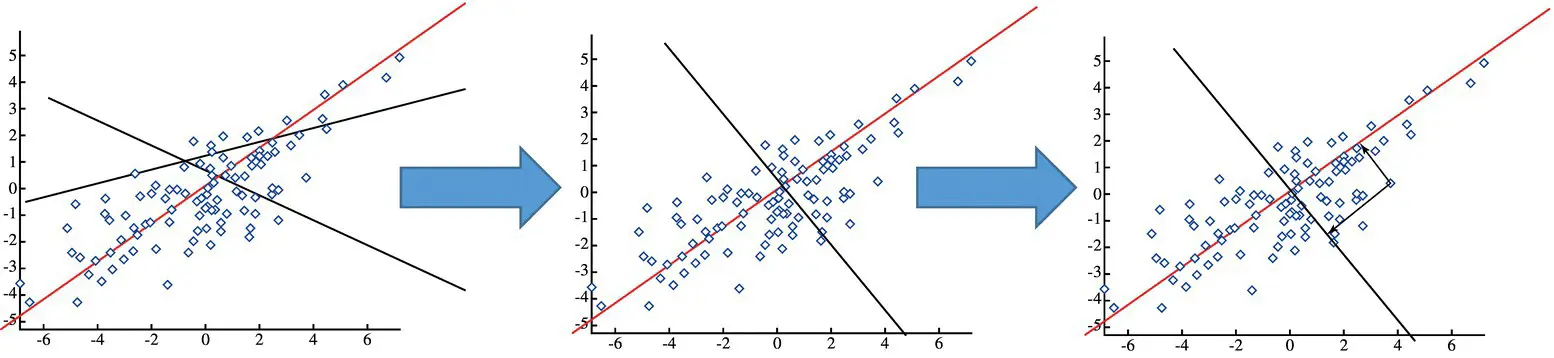
Figure 2.15 Successive data projections.
The full set of PCs comprises a new orthogonal basis for the feature space, whose axes are aligned with the maximum variances of the original data. The projection of original data onto the first k PCs gives a reduced dimensionality representation of the data. Transforming reduced dimensionality projection back into the original space gives a reduced dimensionality reconstruction of the original data. Reconstruction will have some error, but it can be small and often is acceptable given the other benefits of dimensionality reduction. Choosing the dimension k is based on ∑ i = 1,k λ i/ ∑ i = 1,S λ i> β [%], where β is a predetermined value.
2.2 ML Algorithm Analysis
2.2.1 Logistic Regression
In this section, we provide more details on the performance analysis [4] of the logistic regression introduced initially in Section 2.1.2. There, in Eq. (2.5), we provide an expression for the probability that an individual with dataset values X 1, X 2, …, X pis in outcome g . That is, p g= Pr( Y = g ∣ X). For this expression, we need to estimate the parameters β ’ s used in B ’ s . The likelihood for a sample of N observations is given by
(2.7) 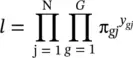
where  and y gjis one if the j thobservation is in outcome g and zero otherwise. Using the fact that
 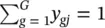 , the log likelihood, L , becomes
(2.8) 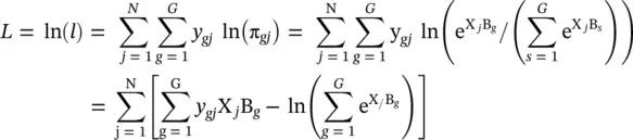
Maximum likelihood estimates of the β’s are those values that maximize this log likelihood equation. This is accomplished by calculating the partial derivatives and setting them to zero. These equations are ∂L / ∂ β ik 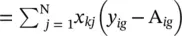 for g = 1, 2, …, G and k = 1, 2, …, p . Since all coefficients are zero for g = 1, the effective range of g is from 2 to G .
Because of the nonlinear nature of the parameters, there is no closed‐form solution to these equations, and they must be solved iteratively. The Newton–Raphson [4–7] method is used to solve these equations. This method makes use of the information matrix, I (β), which is formed from the matrix of second partial derivatives.
The elements of the information matrix are given by 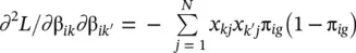
Интервал:
Закладка:
Похожие книги на «Artificial Intelligence and Quantum Computing for Advanced Wireless Networks»
Представляем Вашему вниманию похожие книги на «Artificial Intelligence and Quantum Computing for Advanced Wireless Networks» списком для выбора. Мы отобрали схожую по названию и смыслу литературу в надежде предоставить читателям больше вариантов отыскать новые, интересные, ещё непрочитанные произведения.


Обсуждение, отзывы о книге «Artificial Intelligence and Quantum Computing for Advanced Wireless Networks» и просто собственные мнения читателей. Оставьте ваши комментарии, напишите, что Вы думаете о произведении, его смысле или главных героях. Укажите что конкретно понравилось, а что нет, и почему Вы так считаете.