Savo G. Glisic - Artificial Intelligence and Quantum Computing for Advanced Wireless Networks

For GBM and XGBoost in Python, see [2].

Support vector machine (SVM) is a supervised ML algorithm that can be used for both classification and regression challenges [48, 49]. However, it is mostly used in classification problems. In the SVM algorithm, we plot each data item as a point in n‐dimensional space (where n is the number of features) with the value of each feature being the value of a particular coordinate. Then, we perform classification by finding the hyperplane that differentiates the two classes very well, as illustrated in Figure 2.5.

Support vectors are simply the coordinates of individual observations. The SVM classifier is a frontier that best segregates the two classes (hyperplane Figure 2.5(upper part)/line Figure 2.5(lower part)). The next question is how we identify the right hyperplane. In general, as a rule of thumb, we select the hyperplane that better segregates the two classes, that is,

If multiple choices are available, choose the option that maximizes the distances between nearest data point (either class) and the hyperplane. This distance is called the margin. Figure 2.5 Data classification. Figure 2.6 Classification with outliers.

If the two classes cannot be segregated using a straight line as one of the elements lies in the territory of other class as an outlier (see Figure 2.6), the SVM algorithm has a feature to ignore outliers and find the hyperplane that has the maximum margin. Hence, we can state that SVM classification is robust to outliers.

In some scenarios, we cannot have a linear hyperplane between the two classes. Linear classifiers are not complex enough sometimes. In such cases, SVM maps data into a richer feature space including nonlinear features, and then constructs a hyperplane in that space so that all other equations are identical ( Figure 2.7). Formally, it preprocesses data with: x → Φ(x) and then learns the map from Φ(x) to y as follows:

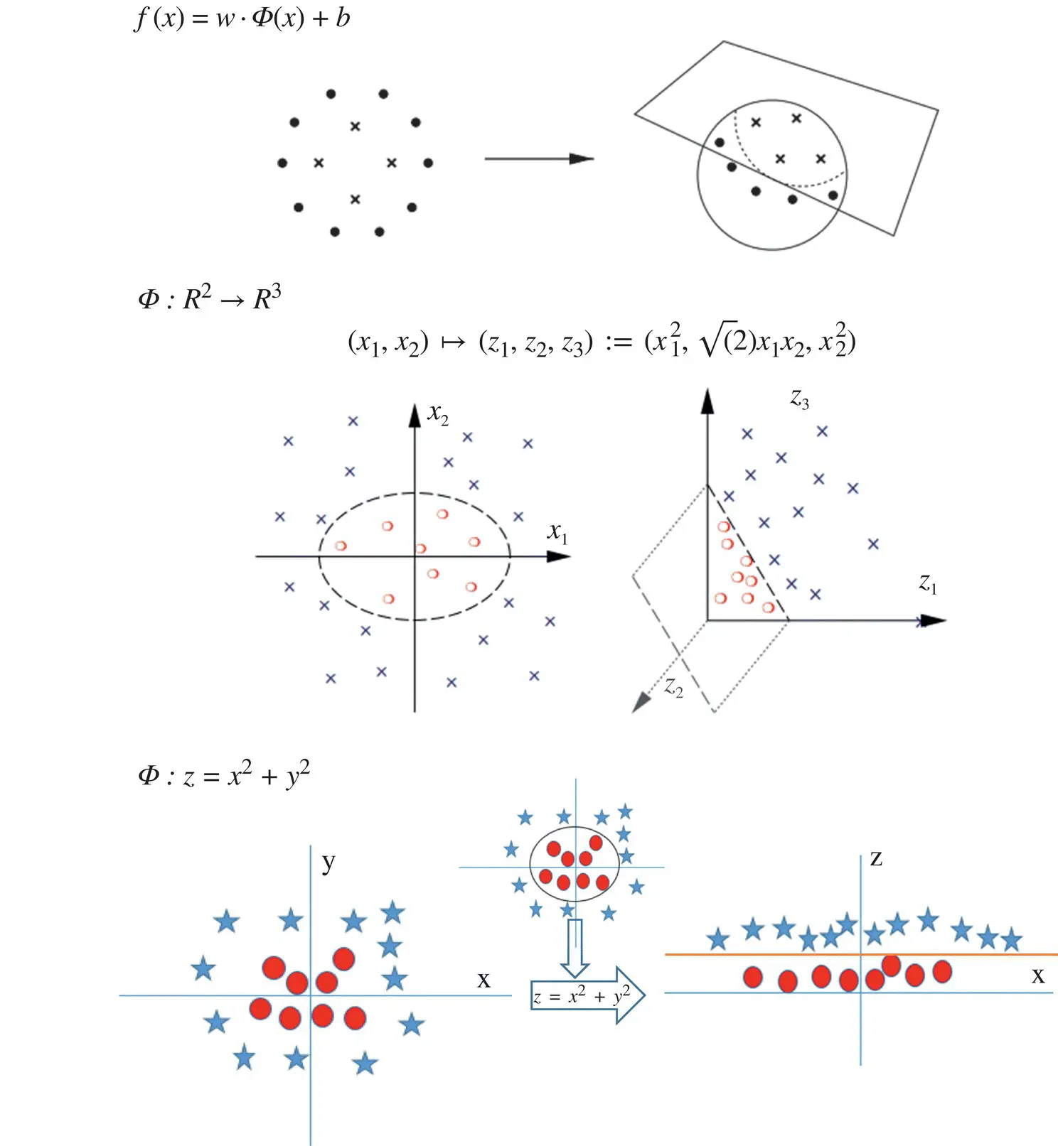
Figure 2.7 Classifiers with nonlinear transformations.

The e1071 package in R is used to create SVMs.

It has helper functions as well as code for the naive Bayes classifier. The creation of an SVM in R and Python follows similar approaches:

#Import Library require(e1071) #Contains the SVM Train <- read.csv(file.choose()) Test <- read.csv(file.choose()) # there are various options associated with SVM training; like changing kernel, gamma and C value. # create model model <- svm(Target~Predictor1+Predictor2+Predictor3,data=Train,kernel='linear',gamma=0.2,cost=100) #Predict Output preds <- predict(model,Test) table(preds)

Naive Bayes algorithm : This is a classification technique based on Bayes’ theorem with an assumption of independence among predictors. In simple terms, a naive Bayes classifier assumes that the presence of a particular feature in a class is unrelated to the presence of any other feature.

An animal may be considered to be a tiger if it has four legs, weighs about 250 pounds, and has yellow fur with black strips. Even if these features depend on each other or upon the existence of the other features, all of these properties independently contribute to the probability that this animal is a tiger, and that is why it is known as “Naive.”

Along with simplicity, Naive Bayes is known to outperform even highly sophisticated classification methods. Bayes’ theorem provides a way of calculating posterior probability P(c|x) from P(c) , P(x) and P(x|c) . Here we start with

(2.6)

where

P(c|x) is the posterior probability of class (c, target) given predictor (x, attributes).

P(c) is the prior probability of the class.

P(x|c) is the likelihood, which is the probability of a predictor given the class.

P(x) is the prior probability of the predictor.

Suppose we observe a street guitar player who plays different types of music, say, jazz, rock, or country . Passersby leave a tip in a box in front of him depending on whether or not they like what he is playing. The player chooses to play different songs independent of the tips he receives. Below we have a training dataset of song and the corresponding target variable “tip” (which suggests possibilities of getting a tip for a given song). Now, we need to classify whether player will get a tip or not based on the song he is playing. Let us follow the steps involved in this task.

1 Convert the dataset into a frequency table Data TablesongjazzrockcountryjazzjazzrockcountrycountryjazztipnoyesyesyesyesyesnonoyescountryjazzrockrockcountryyesnoyesyesnoFrequency Tablesongnoyesrock4country32jazz23sum59

2 Create a Likelihood table by finding the probabilities, for example, rock probability = 0.29 and probability of getting a tip is 0.64.Likelihood Tablesongnoyesrock4=4/140.29country32=5/140.36jazz23=5/140.36sum59=5/14=9/140.360.64

3 Now, use the Naive Bayesian equation to calculate the posterior probability for each class. The class with the highest posterior probability is the outcome of prediction.

In our case, the player will get a tip if he plays jazz. Is this statement correct? We can solve it using the above method of posterior probability.

which has a relatively high probability. On the other hand, if he plays rock we have

R Code for Naive Bayes

require(e1071) #Holds the Naive Bayes Classifier Train <- read.csv(file.choose()) Test <- read.csv(file.choose()) #Make sure the target variable is of a two-class classification problem only levels(Train$Item:Fat_Content) model <- naiveBayes(Item:Fat_Content~., data = Train) class(model) pred <- predict(model,Test) table(pred)

Nearest neighbor algorithms : These are among the “simplest” supervised ML algorithms and have been well studied in the field of pattern recognition over the last century. They might not be as popular as they once were, but they are still widely used in practice, and we recommend that the reader at least consider the k ‐nearest neighbor algorithm in classification projects as a predictive performance benchmark when trying to develop more sophisticated models. In this section, we will primarily talk about two different algorithms, the nearest neighbor (NN) algorithm and the k ‐nearest neighbor ( k NN) algorithm. NN is just a special case of k NN, where k = 1. To avoid making this text unnecessarily convoluted, we will only use the abbreviation NN if we talk about concepts that do not apply to k NN in general. Otherwise, we will use k NN to refer to NN algorithms in general, regardless of the value of k .