Savo G. Glisic - Artificial Intelligence and Quantum Computing for Advanced Wireless Networks

The information matrix is used because the asymptotic covariance matrix of the maximum likelihood estimates is equal to the inverse of the information matrix. That is, I (β) −1. This covariance matrix is used in the calculation of confidence intervals for the regression coefficients, odds ratios, and predicted probabilities.

The interpretation of the estimated regression coefficients is not straightforward. In logistic regression, not only is the relationship between X and Y nonlinear, but also, if the dependent variable has more than two unique values, there are several regression equations. Consider the usual case of a binary dependent variable, Y , and a single independent variable, X . Assume that Y is coded so it takes on the values 0 and 1. In this case, the logistic regression equation is ln ( p /(1 − p )) = β 0+ β 1 X . Now consider impact of a unit increase in X . The logistic regression equation becomes ln ( p ′ /(1 − p ′)) = β 0+ β 1( X + 1) = β 0+ β 1 X + β 1. We can isolate the slope by taking the difference between these two equations. We have

(2.9)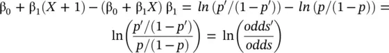

That is, β 1is the log of the ratio of the odds at X + 1 and X . Removing the logarithm by exponentiating both sides gives 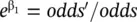. The regression coefficient β 1is interpreted as the log of the odds ratio comparing the odds after a one unit increase in X to the original odds. Note that the interpretation of β1 depends on the particular value of X since the probability values, the p ′ s, will vary for different X .

Inferences about individual regression coefficients, groups of regression coefficients, goodness of fit, mean responses, and predictions of group membership of new observations are all of interest. These inference procedures can be treated by considering hypothesis tests and/or confidence intervals. The inference procedures in logistic regression rely on large sample sizes for accuracy. Two procedures are available for testing the significance of one or more independent variables in a logistic regression: likelihood ratio tests and Wald tests . Simulation studies usually show that the likelihood ratio test performs better than the Wald test. However, the Wald test is still used to test the significance of individual regression coefficients because of its ease of calculation.

The likelihood ratio test statistic is −2 times the difference between the log likelihoods of two models, one of which is a subset of the other. The likelihood ratio is defined as LR = −2[ L subset− L full] = −2[ ln ( l subset/ l full)]. When the full model in the likelihood ratio test statistic is the saturated model, LR is referred to as the deviance . A saturated model is one that includes all possible terms (including interactions) so that the predicted values from the model equal the original data. The formula for the deviance is D = −2[ L Reduced− L Saturated]. The deviance may be calculated directly using the formula for the deviance residuals:

(2.10)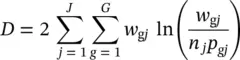

This expression may be used to calculate the log likelihood of the saturated model without actually fitting a saturated model. The formula is L Saturated= L Reduced+ D/2.

The deviance in logistic regression is analogous to the residual sum of squares in multiple regression. In fact, when the deviance is calculated in multiple regression, it is equal to the sum of the squared residuals. Deviance residuals, to be discussed later, may be squared and summed as an alternative way to calculate the deviance D.

The change in deviance, ΔD , due to excluding (or including) one or more variables is used in logistic regression just as the partial F test is used in multiple regression. Many texts use the letter G to represent ΔD , but we have already used G to represent the number of groups in Y . Instead of using the F distribution, the distribution of the change in deviance is approximated by the chi‐square distribution. Note that since the log likelihood for the saturated model is common to both deviance values, ΔD is calculated without actually estimating the saturated model. This fact becomes very important during subset selection. The formula for ΔD that is used for testing the significance of the regression coefficient(s) associated with the independent variable X 1 is ΔD X1= D without X1− D with X1= −2 [L without X1− L Saturated] + 2[ L with X1− L Saturated] = −2[ L withoutX1− L withX1].

Note that this formula looks identical to the likelihood ratio statistic. Because of the similarity between the change in deviance test and the likelihood ratio test, their names are often used interchangeably.

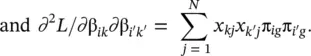
The formula for the Wald statistic is , where is an estimate of the standard error of b jprovided by the square root of the corresponding diagonal element of the covariance matrix, . With large sample sizes, the distribution of z jis closely approximated by the normal distribution. With small and moderate sample sizes, the normal approximation is described as “adequate.”

As indicated in Section 2.1, decision trees are considered to be one of the most popular approaches for representing classifiers. Here, we present a number of methods for constructing decision tree classifiers in a top‐down manner. This section suggests a unified algorithmic framework for presenting these algorithms and describes the various splitting criteria and pruning methodologies. The material is discussed along the lines presented in [8–11].

Supervised methods are methods that attempt to discover relationship between the input attributes and the target attribute. The relationship discovered is represented in a structure referred to as a model. Usually, models can be used for predicting the value of the target attribute knowing the values of the input attributes. It is useful to distinguish between two main supervised models: classification models (classifiers) and regression models. Regression models map the input space into a real‐valued domain, whereas classifiers map the input space into predefined classes. For instance, classifiers can be used to classify students into two groups: those passing exams on time and those passing exams with a delay. Many approaches are used to represent classifiers. The decision tree is probably the most widely used approach for this purpose.