Savo G. Glisic - Artificial Intelligence and Quantum Computing for Advanced Wireless Networks

k NN is an algorithm for supervised learning that simply stores the labeled training examples, 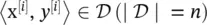, during the training phase and postpones the processing of the training examples until the phase of making predictions. Again, the training consists literally of just storing the training data.

Then, to make a prediction (class label or continuous target), the kNN algorithms find the k nearest neighbors of a query point and compute the class label (classification) or continuous target (regression) based on the k nearest (most “similar”) points. The overall idea is that instead of approximating the target function f (x) = y globally, during each prediction, k NN approximates the target function locally. In practice, it is easier to learn to approximate a function locally than globally.

Figure 2.8illustrates the NN classification algorithm in two dimensions (features x 1and x 2). In the left subpanel, the training examples are shown as blue dots, and a query point that we want to classify is shown as a question mark. In the right subpanel, the class labels are also indicated, and the dashed line indicates the nearest neighbor of the query point, assuming a Euclidean distance metric. The predicted class label is the class label of the closest data point in the training set (here: class 0).

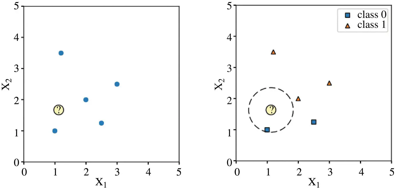
Figure 2.8 Illustration of the nearest neighbor (NN) classification algorithm in two dimensions (features x 1and x 2).

More formally, we can define the 1‐NN algorithm as follows:

Training algorithm: for i = 1, n in the n ‐dimensional training data set D ∣ D ∣ = n : •store training example 〈x [i], f(x [i])〉 Prediction algorithm: closest point≔ None closest distance≔∞ •for i = 1, n: ‐current distance≔d(x [i], x [q]) ‐if current distance < closest distance: * closest distance≔ current distance * closest point≔x [i] prediction h(x [q]) is the target value of closest point

Unless noted otherwise, the default distance metric (in the context of this section) of NN algorithms is the Euclidean distance (also called L 2distance), which computes the distance between two points, x [a]and x [b]:

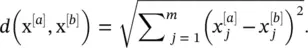
Decision boundary: Assuming a Euclidean distance metric, the decision boundary between any two training examples a and b is a straight line. If a query point is located on the decision boundary, this implies its equidistance from both training example a and b. Although the decision boundary between a pair of points is a straight line, the decision boundary of the NN model on a global level, considering the whole training set, is a set of connected, convex polyhedra. All points within a polyhedron are closest to the training example inside, and all points outside the polyhedron are closer to a different training example. Figure 2.9illustrates the plane partitioning of a two‐dimensional dataset (features x 1and x 2) via linear segments between two training examples (a & b, a & c, and c & d) and the resulting Voronoi diagram (lower‐right corner).

Figure 2.9 Illustration of the plane partitioning of a two‐dimensional dataset.

This partitioning of regions on a plane in 2D is also called a Voronoi diagram or Voronoi tessellation. Given a discrete set of points, a Voronoi diagram can also be obtained by a process known as Delaunay triangulation by connecting the centers of the circumcircles.

Whereas each linear segment is equidistant from two different training examples, a vertex (or node) in the Voronoi diagram is equidistant from three training examples. Then, to draw the decision boundary of a two‐dimensional NN classifier, we take the union of the pair‐wise decision boundaries of instances of the same class. An illustration of the NN decision boundary as the union of the polyhedra of training examples belonging to the same class is shown in Figure 2.10.

k‐Means clustering: In this section, we will cover k‐means clustering and its components. We will look at clustering, why it matters, and its applications, and then dive into k‐means clustering (including how to perform it in Python on a real‐world dataset).

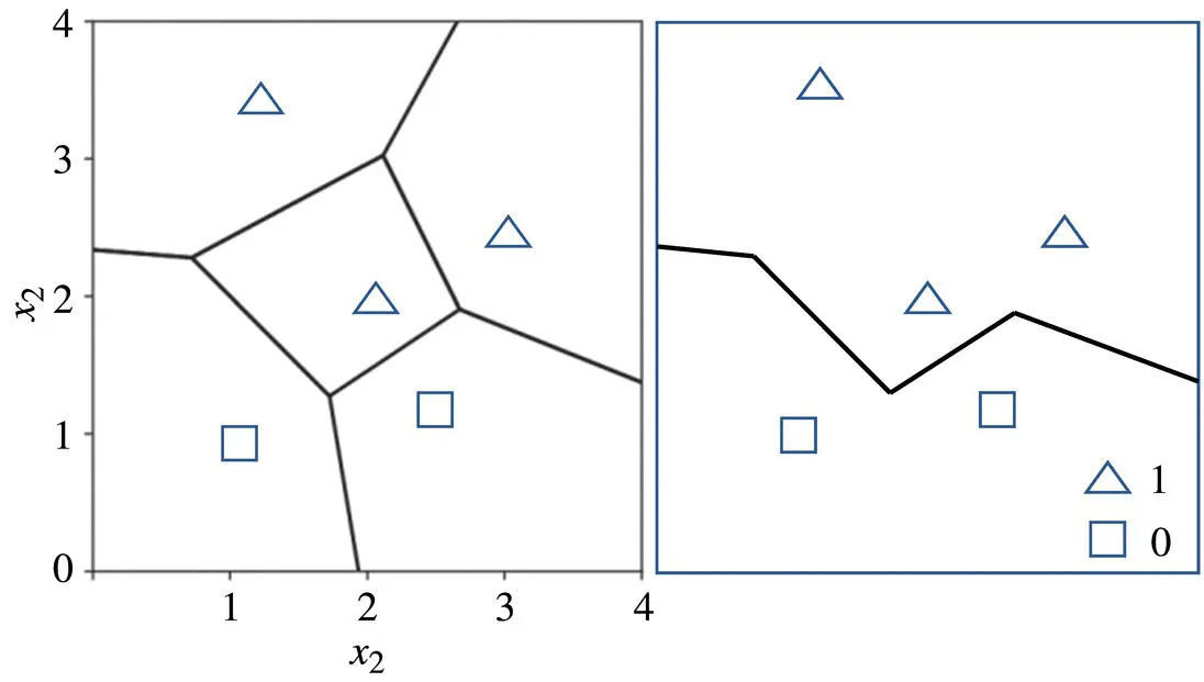
Figure 2.10 Illustration of the nearest neighbor (NN) decision boundary.

A university wants to offer to its customers (companies in industry) new continuous education type of courses. Currently, they look at the details of each customer and based on this information, decide which offer should be given to which customer. The university can potentially have a large number of customers. Does it make sense to look at the details of each customer separately and then make a decision? Certainly not! It is a manual process and will take a huge amount of time. So what can the university do? One option is to segment its customers into different groups. For instance, each department of the university can group the customers for their field based on their technological level (tl; general education background of the employees), say, three groups high (htl), average (atl), and low (ltl). The department can now draw up three different strategies (courses of different level of details) or offers, one for each group. Here, instead of creating different strategies for individual customers, they only have to formulate three strategies. This will reduce the effort as well as the time.

The groups indicated in the example above are known as clusters, and the process of creating these groups is known as clustering. Formally, we can say that clustering is the process of dividing the entire data into groups (also known as clusters) based on the patterns in the data. Clustering is an unsupervised learning problem! In these problems, we have only the independent variables and no target/dependent variable. In clustering, we do not have a target to predict. We look at the data and then try to club similar observations and form different groups. Hence, it is an unsupervised learning problem.

In order to discuss the properties of the cluster, let us further extend the previous example to include one more characteristic of the customer:

We will take the same department as before that wants to segment its customers. For simplicity, let us say the department wants to use only the technological level ( tl ) and background mismatch ( bm ) to make the segmentation. Background mismatch is defined as the difference between the content of the potential course and the technical expertise of the customer. They collected the customer data and used a scatter plot to visualize it (see Figure 2.11):

Now, the department can offer a rather focused, high‐level course to cluster C 4since the customer employees have high‐level general technical knowledge with expertise that is close to the content of the course. On the other hand, for cluster C 1, the department should offer a course on the broader subject with fewer details.