Savo G. Glisic - Artificial Intelligence and Quantum Computing for Advanced Wireless Networks

3 They all have the same variance (“homoscedasticity”).

4 They are normally distributed.

These assumptions will never be exactly satisfied by real data, but you hope that they are not badly wrong. For proper regression modeling, we need to collect data that are relevant and informative with respect to our decision problem, and then define the variables and construct the model in such a way that the assumptions listed above are plausible, at least as a first‐order approximation to reality.

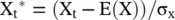
If we normalize the values of Y and X as

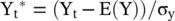
with the correlation function defined as

the phenomenon that Galton noted was that the regression line for predicting Y* from X* passes through the origin and has a slope equal to the correlation between Y and X; that is, the regression equation in normalized units is

Figures 2.1and 2.2illustrate this equation [1]. When the units of X and Y are standardized and both are also normally distributed, their values are distributed in an elliptical pattern that is symmetric around the 45° line, which has a slope equal to 1.

However, the regression line for predicting Y* from X* is not the 45° line. Rather, it is a line passing through the origin whose slope is r XY, the dashed gray line in the picture below, which is tilted toward the horizontal because the correlation is less than 1 in magnitude. In other words, it is a line that “regresses” (i.e. moves backward) toward the X‐axis.

Logistic regression analysis studies the association between a categorical dependent variable and a set of independent (explanatory) variables. The term logistic regression is used when the dependent variable has only two values, such as 0 and 1, or Yes and No. Suppose the numerical values of 0 and 1 are assigned to the two outcomes of a binary variable. Often, 0 represents a negative response, and 1 represents a positive response. The mean of this variable will be the proportion of positive responses. If p is the proportion of observations with an outcome of 1, then 1 − p is the probability of a outcome of 0. The ratio p /(1 − p ) is called the odds and the logit is the logarithm of the odds, or just log odds . Formally, the logit transformation is written as l = logit ( p ) = ln ( p /(1 − p )). Note that while p ranges between 0 and 1, the logit ranges between minus and plus infinity. Also, note that the zero logit occurs when p is 0.50. The logistic transformation is the inverse of the logit transformation. It is written as p = logistic( l ) = e l/(1 + e l)

The difference between two log odds can be used to compare two proportions, such as that of boys versus girls. Formally, this difference is written as

(2.3)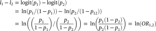

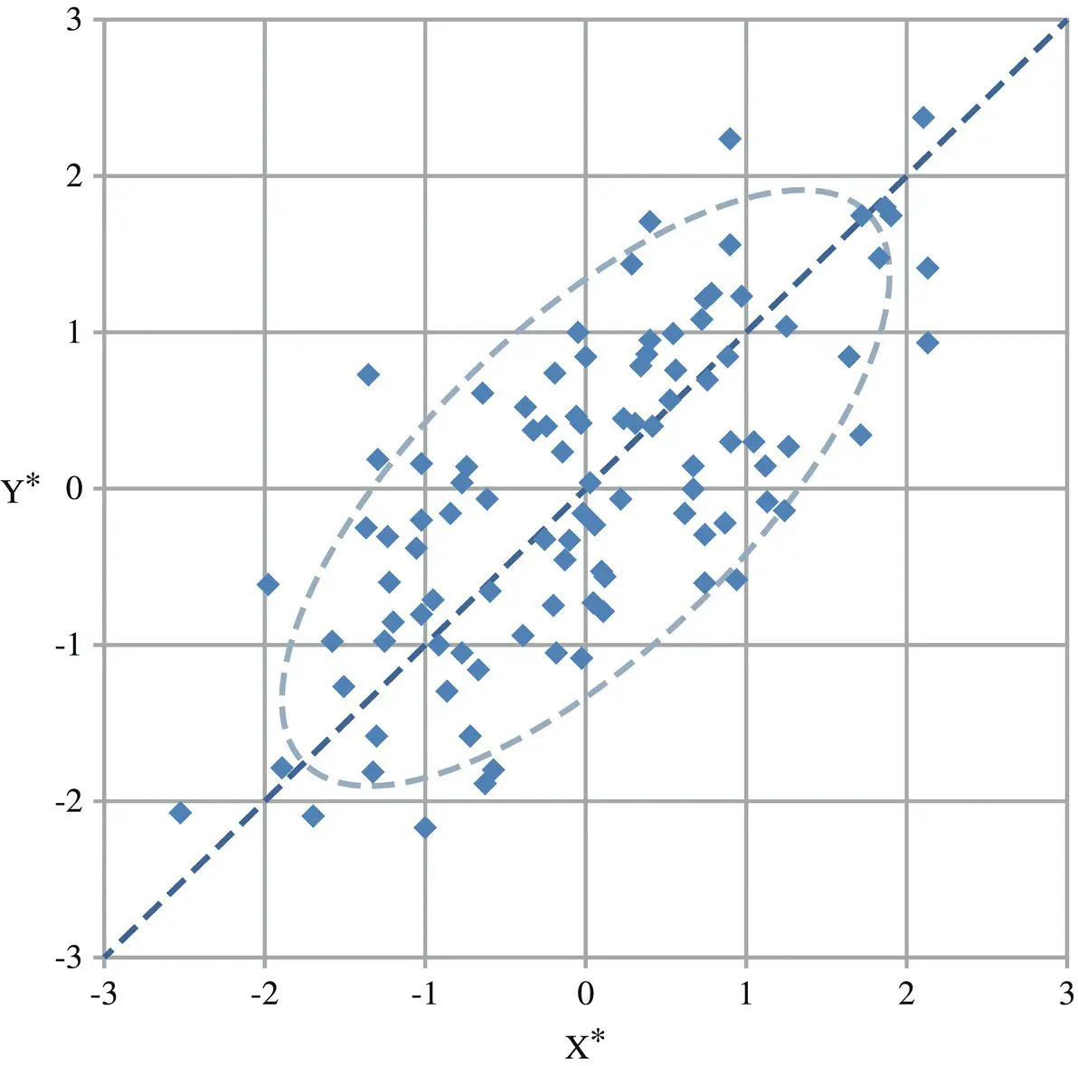
Figure 2.1 If X and Y are two jointly normally distributed random variables, then in standardized units (X*, Y*) their values are scattered in an elliptical pattern that is symmetric around the 45° line.

Source: Modified from Introduction to linear regression analysis [50]. Available at https://people.duke.edu/~rnau/regintro.htm.

This difference is often referred to as the log odds ratio . The odds ratio is often used to compare proportions across groups. Note that the logistic transformation is closely related to the odds ratio. The converse relationship is

(2.4)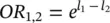

In logistic regression, a categorical dependent variable Y having G (usually G = 2) unique values is regressed on a set of p independent variables X 1, X 2, …, X p.

Let X = ( X 1, X 2, …, X p) and B g= ( β g1, …, β gp) T; then the logistic regression model is given by the G equations ln ( p g /p 1) = ln ( P g /P 1) + β g1 X 1+ β g2 X 2+ …. + β gp X p= ln ( P g/ P 1) + XB g. Here, p gis the probability that an individual with values X 1, X 2, …, X pis in outcome g . That is, p g= Pr( Y = g ∣ X). Usually, X 1≡ 1 (that is, an intercept is included), but this is not necessary. The quantities P 1, P 2, …, P Grepresent the prior probabilities of outcome membership. If these prior probabilities are assumed equal, then the term ln ( P g/ P 1) becomes zero and drops out. If the priors are not assumed equal, they change the values of the intercepts in the logistic regression equation.

The first outcome is called the reference value . The regression coefficients β 1 , β 2 , …, β pfor the reference value are set to zero. The choice of the reference value is arbitrary. Usually, it is the most frequent value or a control outcome to which the other outcomes are to be compared. This leaves G − 1 logistic regression equations in the logistic model.

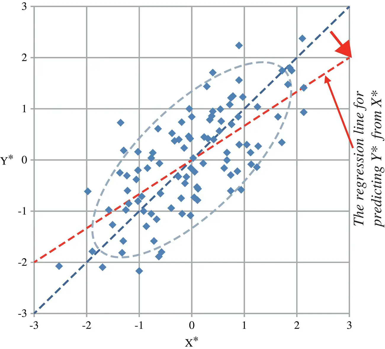
Figure 2.2 The regression line for predicting Y* from X* is not the 45° line. It has slope rXY, which is less than 1. Hence it “regresses” toward the X‐axis. For this data sample, rXY = 0.69.

The β’ s are population regression coefficients that are to be estimated from the data. Their estimates are represented by b ’s. The β’ s represent unknown parameters to be estimated, whereas the b ’s are their estimates. These equations are linear in the logits of p . However, in terms of the probabilities, they are nonlinear. The corresponding nonlinear equations are

(2.5)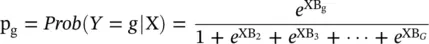

since because all of its regression coefficients are zero. Using the fact that e a + b= ( e a)( e b), e XBmay be reexpressed as follows: e XB= exp(β 1 X 1+ β 2 X 2+ ⋯ + β ρ X p) = e β1 X1 e β2 X2 …e βp Xp . This shows that the final value is the product of its individual terms.