Neil McCartney - Properties for Design of Composite Structures

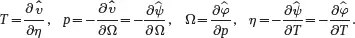
and the differential relations ( 2.63) reduce to the simpler forms

(2.68)

whereas relations ( 2.66) reduce to

(2.69)

The analysis of this section has been presented as it establishes a basis for connecting composite modelling to the well-known principles of thermodynamics. The relationships ( 2.67)–( 2.69) apply to single-component solids subject only to hydrostatic stress states leading to the possibility of specifying constitutive equations that depend on a limited set of material properties, e.g. bulk modulus and bulk thermal expansion coefficient. To extend the analysis to all types of thermoelastic material properties needed for the applications to be considered in this book, it is required to introduce in the next section strain tensors as state variables, rather than the specific volume Ω introduced in ( 2.65) and ( 2.67).

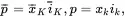
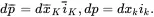
Unlike the situation for fluids, the deformation (i.e. motion) of solid media is defined relative to an initial homogeneous reference state, thus enabling the introduction of the concept of strain, which takes account of both hydrostatic deformation considered in Section 2.9 and shear deformation. Following the approach in [1], consider now a homogeneous solid body with an initial configuration that occupies a region B¯, and which deforms into a different region B after the application of applied stresses and temperature changes. Let p¯ denote the position vector of some point in the undeformed body B¯ referred to Cartesian coordinates x¯, that moves to the point pin the deformed body B referred to Cartesian coordinates x. Let i¯K denote the orthogonal unit base vectors for the coordinate system x¯, and ik denote the orthogonal unit base vectors for the coordinate system x. The position vectors p¯ and pmay then be expressed in the following form

(2.70)

where summations over values K , k = 1, 2, 3, are implied for repeated suffices. The corresponding infinitesimal vectors are written as

(2.71)

As

(2.72)

it follows that

(2.73)

Any vector vmay be written as

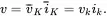(2.74)

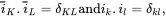
Define δKl and δkL by the relation

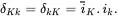(2.75)

It then follows that

(2.76)

It is clear that

(2.77)

The time-dependent deformation that transforms the undeformed region B¯ into the region B( t ) may be expressed as

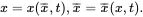(2.78)

It then follows that

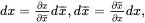(2.79)

where the increments are taken at some time t such that d t = 0. In component form,

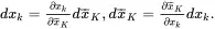(2.80)

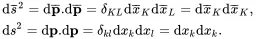
In the undeformed body, on using ( 2.71) and ( 2.73), the increment of arc length ds¯ is such that

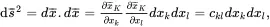(2.81)

where ckl is Cauchy’s symmetric deformation tensor. Similarly, for the deformed body, the line increment ds¯deforms to an increment ds such that

(2.82)

where CKL is Green’s symmetric deformation tensor. In dyadic form

(2.83)

where ∇¯ denotes the gradient with respect to the material coordinates x¯, and where the symmetric Green deformation tensor Cmay be written as

(2.84)

From ( 2.81) and ( 2.82)

(2.85)

The Eulerian and Lagrange strain tensors are defined by

(2.86)

so that ( 2.85) may also be written as

(2.87)

On using the relation u=x−x¯ for the displacement vector and ( 2.84), the Lagrangian strain tensor may be written in terms of the displacement vector as follows

(2.88)

where Iis the symmetric fourth-order identity tensor (see ( 2.15)). The quantity Eis the strain tensor that is used in finite deformation theory where there is no restriction on the degree of deformation provided that the deformation is continuous and the condition ( 2.18) is satisfied at all points in the system.