William M. White - Geochemistry

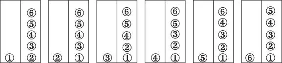
Figure 2.7 There are six possible ways to distribute six energy units so that the left block has one unit and the right block has five units.

(2.36) †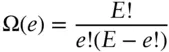

Here we use Ω(e) to denote the function that describes the number of states accessible to the system for a given value of e . In this particular example, “states accessible to the system” refers to a given distribution of energy units between the two blocks. According to eqn. 2.36there are 20 ways of distributing our six units of energy so that each block has three. There is, of course, only one way to distribute energy so that the left block has all of the energy and only one combination where the right block has all of it.

According to the basic postulate, any of the 64 possible distributions of energy are equally likely. The key observation, however, is that there are many ways to distribute energy for some values of e and only a few for other values. Thus the chances of the system being found in a state where each block has three units is 20/64 = 0.3125, whereas the chances of the system being in the state with the original distribution (one unit to the left, five to the right) are only 6/64 = 0.0938. So it is much more likely that we will find the system in a state where energy is equally divided than in the original state.

Of course, two macroscopic blocks of copper at any reasonable temperature will have far more than 6 quanta of energy. Let's take a just slightly more realistic example and suppose that they have a total of 20 quanta and compute the distribution. There will be 220 possible distributions, far too many to consider individually, so let's do it the easy way and use eqn. 2.36to produce a graph of the probability distribution. Equation 2.36gives the number of identical states of the system for a given value of e . The other thing that we need to know is that the chances of any one of these states occurring is simply (1/2) 20. So to compute the probability of a particular distinguishable distribution of energy occurring, we multiply this probability by Ω. More generally, the probability, P , will be:

(2.37)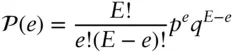

where p is the probability of an energy unit being in the left block and q is the probability of it being in the right. This equation is known as the binomial distribution . §Since both p and q are equal to 0.5 in our case (if the blocks were of different mass or of different composition, p and q would not be equal), the product p e q E–eis just p Eand eqn. 2.37simplifies to:

(2.38)

Since p Eis a constant (for a given value of E and configuration of the system), the probability of the left block having e units of energy is directly proportional to Ω( e ). It turns out that this is a general relationship, so that for any system we may write:

(2.39)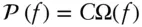

where ƒ is some property describing the system and C is some constant (in this case 0.5 20). Figure 2.8a shows the probability of the left block having e units of energy. Clearly, the most likely situation is that both will have approximately equal energy. The chance of one block having 1 unit and the other 19 units is very small (2 × 10 −5to be exact). In reality, of course, the number of quanta of energy available to the two copper blocks will be of the order of multiples of the Avogadro number. If one or the other block has 10 or 20 more units or even 10 10more quanta than the other, we wouldn't be able to detect it. Thus, energy will always appear to be distributed evenly between the two, once the system has had time to adjust.

Figure 2.8b shows Ω as a function of e , the number of energy units in the left block. Comparing the two, as well as eqn. 2.38, we see that the most probable distribution of energy between the blocks corresponds to the situation where the system has the maximal number of states accessible to it (i.e., to where Ω(e) is maximum).

According to our earlier definition of equilibrium, the state ultimately reached by this system when we removed the constraint (the insulation) is the equilibrium one. We can see here that, unlike the ball on the hill, we cannot determine whether this system is at equilibrium or not simply from its energy: the total energy of the system remained constant. In general, for a thermodynamic system, whether the system is at equilibrium depends not on its total energy but on how that energy is internally distributed .

Clearly, it would be useful to have a function that could predict the internal distribution of energy at equilibrium. The function that does this is the entropy . To understand this, let's return to our copper blocks. Initially, a thermal barrier separates the two copper blocks and we can think of each as an isolated system. We assume that each has an internal energy distribution that is at or close to the most probable one (i.e., each is internally at equilibrium). Each block has its own function Ω (which we denote as Ω land Ω rfor the left and right block, respectively) that gives the number of states accessible to it at a particular energy distribution. We assume that initial energy distribution is not the final one, so that when we remove the insulation, the energy distribution of the system will spontaneously change. In other words:

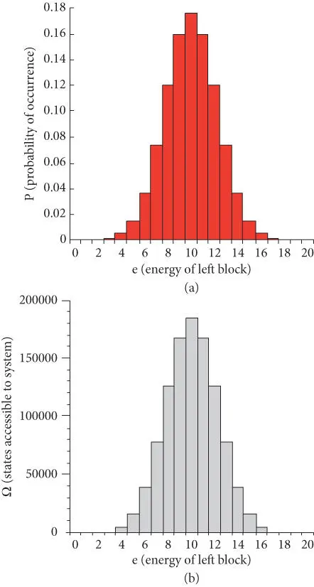
Figure 2.8 (a) Probability of one of two copper blocks of equal mass in thermal equilibrium having e units of energy when the total energy of the two blocks is 20 units. (b) Ω, number of states available to the system (combinations of energy distribution) as a function of e .

where we use the superscripts i and f to denote initial and final, respectively.

When the left block has energy e , it can be in any one of Ω l= Ω( e ) possible states, and the right block can be in any one of Ω r= Ω( E−e ) states. Both and Ω are multiplicative, so the total number of possible states after we remove the insulation, Ω, will be:

To make and Ω additive, we simply take the log: