Michael Begon - Ecology

The desire to formulate general rules in ecology often finds its expression in the construction of mathematical or graphical models. It may seem surprising that ecologists interested in the natural living world should spend time reconstructing it in an artificial mathematical form. But there are several good reasons why this should be done. The first is that models can crystallise, or at least bring together in terms of a few parameters, the important, shared properties of a wealth of unique examples. This simply makes it easier for ecologists to think about the problem or process under consideration, by forcing us to try to extract the essentials from complex systems. Thus, a model can provide a ‘common language’ in which each unique example can be expressed; and if each can be expressed in a common language, then their properties relative to one another, and relative perhaps to some ideal standard, will be more apparent.

Even more important, models can shed light on the real world that they mimic. They can exhibit properties that the system being modelled had not previously been known to possess, and they can make it clear how the behaviour of a population, for example, depends on the properties of the individuals that comprise it. Models do this because they force us to make explicit any assumptions that we choose to make, and mathematical methods are designed precisely to allow a set of assumptions to be followed through to their natural conclusions. We can ask, for example, ‘If only juveniles migrate, what would this do to the dynamics of their populations?’. As a consequence, models often suggest what would be the most profitable experiments to carry out or observations to make – ‘Since juvenile migration rates appear to be so important, these should be measured in each of our study populations’.

These ideas are more familiar, perhaps, in other contexts, but are equally valid in ecology. Other than in their imaginations, Newton never laid hands on a perfectly frictionless body, and Boyle never saw an ideal gas. But Newton’s Laws of Motion and Boyle’s Law have been of immeasurable value to us for centuries.

These reasons for constructing models are also criteria by which any model should be judged. Indeed, a model is only useful (i.e. worth constructing) if it does perform one or more of these functions. Of course, in order to perform them a model must adequately describe real situations and real sets of data, and this ‘ability to describe’ or ‘ability to mimic’ is itself a further criterion by which a model can be judged. However, the crucial word is ‘adequate’. The only perfect description of the real world is the real world itself. A model is an adequate description, ultimately, as long as it performs a useful function.

In the present case, some simple models of intraspecific competition will be described. They will be built up from a very elementary starting point, and their properties (i.e. their ability to satisfy the criteria described above) will then be examined. Initially, a model will be constructed for a population with discrete breeding seasons.

In Section 4.7we developed a simple model for species with discrete breeding seasons, in which the population size at time t, N t, altered in size under the influence of a fundamental net reproductive rate, R . This model can be summarised in two equations:

(5.7)

and:

(5.8)

no competition: exponential growth

The model, however, describes a population in which there is no competition. R is constant, and if R > 1, the population will continue to increase in size indefinitely (‘exponential growth’, shown in Figure 5.20a).

Figure 5.20 Mathematical models of population increase.(a) In populations with discrete generations population increases with time: exponential increase (left) and sigmoidal increase (right). (b) The simplest, straight‐line way in which the inverse of generation increase ( N t/ N t+1) might rise with density ( N t) offers a way of adding competition to exponential increase. For further explanation, see text.

incorporating competition

The first step is therefore to modify the equations by making the net reproductive rate subject to intraspecific competition. This is done in Figure 5.20b, which has three components. At point A, the population size is very small ( N tis virtually zero). Competition is therefore negligible, and the net reproductive rate is adequately defined by an unmodified R . Thus, Equation 5.7is still appropriate, or, rearranging the equation:

(5.9)

At point B, by contrast, the population size ( N t) is very much larger and there is a significant amount of intraspecific competition, such that the net reproductive rate has been so modified by competition that the population can collectively do no better than replace itself each generation, because ‘births’ equal ‘deaths’. In other words, N t+1is simply the same as N t, and N t/ N t+1equals 1. The population size at which this occurs is, by definition, the carrying capacity, K (see Figure 5.13).

The third component of Figure 5.20b is the straight line joining point A to point B and extending beyond it. This describes the progressive modification of the net reproductive rate as population size increases; but its straightness issimply an assumption made for the sake of expediency, since all straight lines are of the simple form: y = (slope) x + (intercept). In Figure 5.21b, N t/ N t+1is measured on the y ‐axis, N ton the x ‐axis, the intercept is 1/ R and the slope, based on the segment between points A and B, is (1 − 1/ R )/ K . Thus:

(5.10)

or, rearranging:

(5.11)

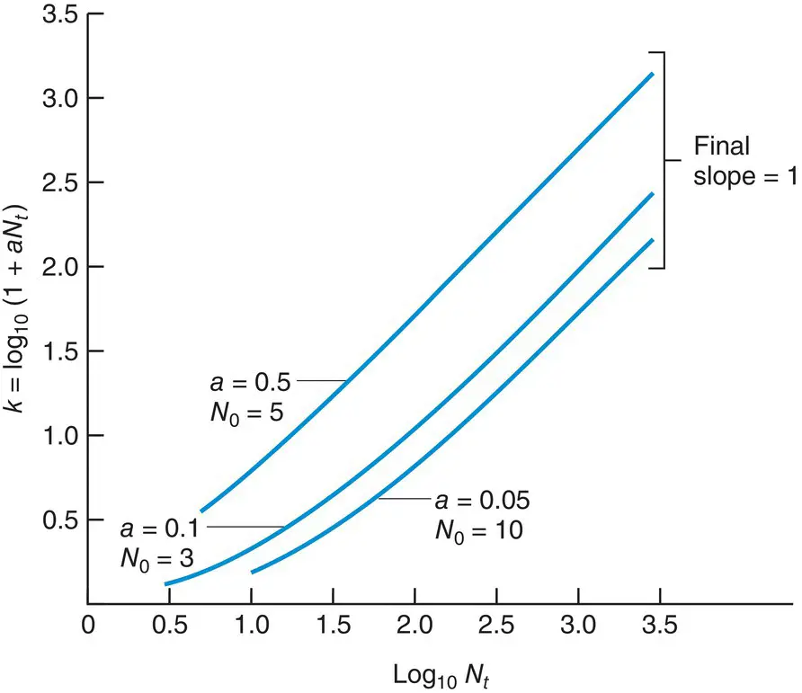
Figure 5.21 The intraspecific competition inherent in Equation 5.13 . The final slope of k against log 10 N tis unity (exact compensation), irrespective of the starting density N 0or the constant a (= ( R − 1)/ K ).

a simple model of intraspecific competition

For further simplicity, ( R − 1)/ K may be denoted by a giving:

(5.12)