Michael Begon - Ecology

Source : After Pearl (1928) and Deevey (1947).

In a type 1 survivorship curve, mortality is concentrated toward the end of the maximum life span. It is perhaps most typical of humans in developed countries and their carefully tended zoo animals and pets. A type 2 survivorship curve is a straight line signifying a constant mortality rate from birth to maximum age. It describes, for instance, the survival of buried seeds in a seed bank. In a type 3 survivorship curve there is extensive early mortality, but a high rate of subsequent survival. This is typical of species that produce many offspring. Few survive initially, but once individuals reach a critical size, their risk of death remains low and more or less constant. This appears to be the most common survivorship curve among animals and plants in nature.

These types of survivorship curve are useful generalisations, but in practice, patterns of survival are usually more complex. We saw with the marmots, for example, that survivorship was broadly type 2 throughout much of their lives, but not at the end ( Figure 4.10b). Similarly, with the dinosaurs we will meet in the next section, survivorship followed the typical type 3 pattern until they reached sexual maturity, but again failed to conform to such a simple classification thereafter (see Figure 4.13). More generally, we see examples approximating to each of the three types in the survey in Figure 4.2, but also more examples where the shape changes as individuals pass through the different phases of their lives.

Opinions naturally differ regarding both the ethics and the practical benefits of keeping wild animals in captivity in zoos, but the current reality is that zoos play an integral role in the conservation of many species, especially those, like many mammals, that are large and inherently attractive to the general public. Hence, in managing these animals, we need to understand their patterns of survivorship, and to know in particular if there are general rules organising these patterns that would not only describe the species for which we have good data, but also allow us to predict patterns for similar or related species when currently available data are sparse. Lynch et al . (2010) therefore reviewed what was known about the survivorship of captive mammals – 37 species, including primates, artiodactyls (cattle, sheep, deer, etc.), carnivores, bats, seals and the giant panda – and some of their results are summarised in Figure 4.12. They were more interested in the shapes of the survivorship curves (and for example whether they were type 1, 2 or 3) than in absolute values, and all data sets were therefore scaled to the maximum longevity of the species concerned. They then fitted all datasets to a general survivorship function with two shape parameters, α and β, which allowed the different curves to be classified and either grouped together or distinguished ( Figure 4.12). Broadly speaking, with increasing values of α/β, mortality shifted towards being more evenly distributed throughout life, rather than being concentrated at the start; and with decreasing values of αβ, mortality shifted towards including senescence – a period of increased mortality at the end of life – rather than decreasing steadily with age.

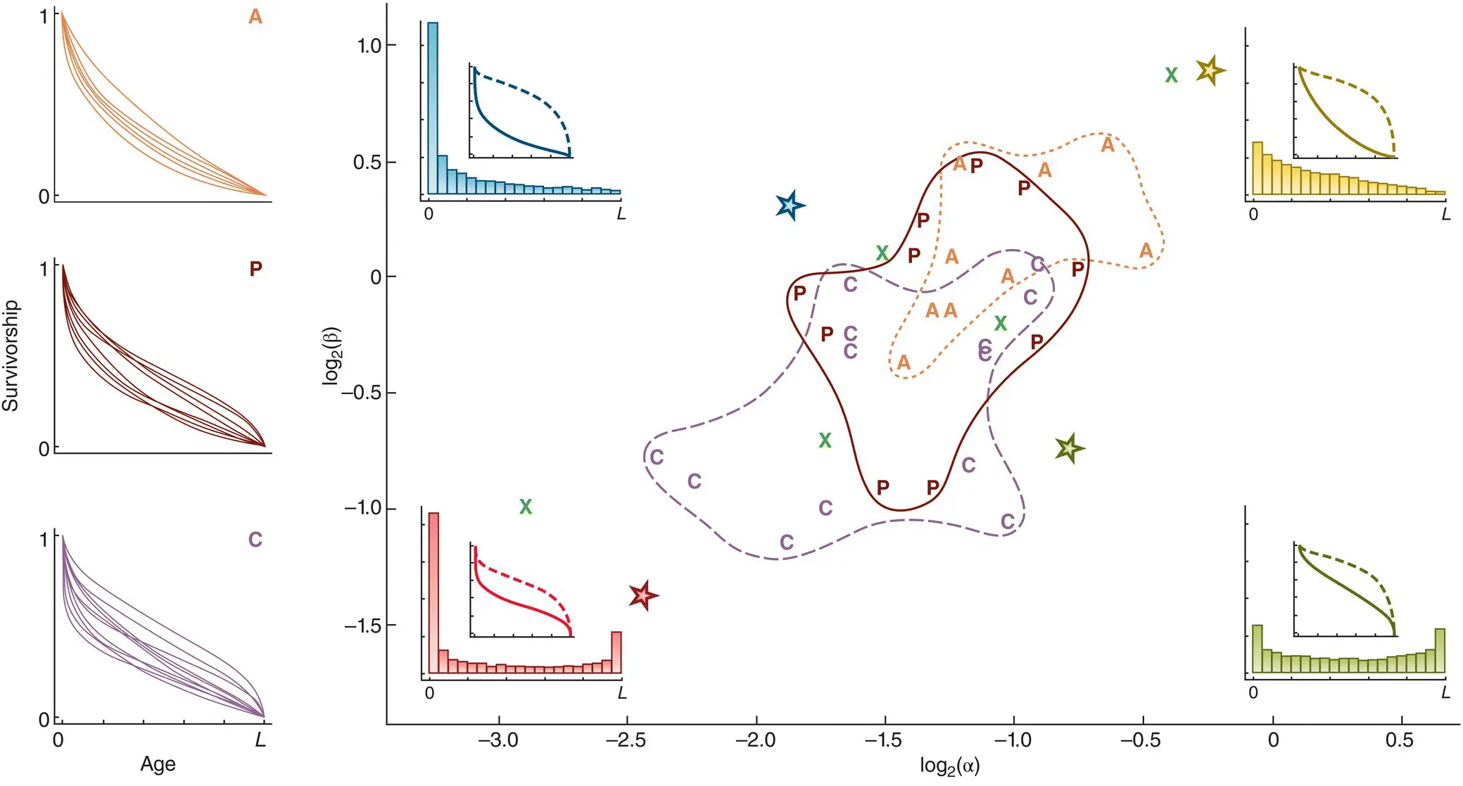
Figure 4.12 Distribution of the shapes of survivorship curves for 37 species of animals kept in zoos.(For a full list of species names, see the original text.) A generalised survivorship function with two parameters, α and β was fitted to all datasets, allowing each to be located in logα–logβ space. The shapes themselves are illustrated in the insets, referring to the four starred locations, as survivorship on linear and semilogarithmic scales (solid and dashed lines, respectively; see Figure 4.11) and as distributions of mortality (histograms) between birth and maximum longevity (L). Among those species, the locations of artiodactyls ( ), carnivores ( ) and primates ( ) are indicated, plus five further species ( ).

Source : After Lynch et al . (2010).

Despite wide variations in size, longevity and taxonomic affiliation, most of the curves were, in essence, type 2, with some element of type 1 (senescence) or type 3 (early mortality). The variation that did exist was significantly associated with the species’ taxonomic order: the artiodactyls showed the least evidence of senescence, the carnivores the most, with the primates somewhere in between ( Figure 4.12). This taxonomic variation was in turn associated with variations in age to weaning (relative to lifespan) and litter size, suggesting ‘syndromes’ of associated life history traits. We return to the whole topic of the patterns in life histories and their possible causes in the next chapter. For now, though, the results do provide us with grounds for believing that, based on this analysis, even for species where we have little or no prior knowledge, managers in zoos can make educated predictions with some confidence about likely patterns of mortality, and act accordingly.

Many of the species that ecologists study, and for which life tables would therefore be valuable, have repeated breeding seasons like the marmots, or continuous breeding as in the case of humans, but constructing life tables here is complicated, largely because these populations have individuals of many different ages living together. Building a cohort life table is sometimes possible, as we have seen, but this is relatively uncommon. Apart from the mixing of cohorts in the population, it can be difficult simply because of the longevity of many species.

useful – if used with caution

Another approach is to construct a static life table ( Figure 4.9). The data look like a cohort life table – a series of different numbers of individuals in different age classes – but these come simply from the age structure of the population captured at one point in time. Hence, great care is required: they can only be treated and interpreted in the same way as a cohort life table if patterns of birth and survival in the population have remained much the same since the birth of the oldest individuals – and this will happen only rarely. Nonetheless, there is often no alternative and useful insights can still be gained. This is illustrated for a population of small dinosaurs, Psittacosaurus lujiatunensis , recovered as fossils from the Lower Cretaceous Yixian Formation in China, where the alternative of following a cohort is obviously not available ( Figure 4.13). They appear to have perished simultaneously in a volcanic mudflow, which might therefore have captured a representative snapshot of the population at the time, around 125 million years ago.

Figure 4.13 Static life tables can be informative, especially when alternatives are not available.(a) The age structure (and hence the static life table) of a population of dinosaurs, Psittacosaurus lujiatunensis , recovered as fossils from the Lower Cretaceous Yixian Formation in China. Age was estimated from the length of the femur, which had been shown in a subsample of specimens to correlate very strongly with the number of ‘growth lines’ (one per year) in the bone. (b) A survivorship curve (log( l x) plotted against age) derived from the life table.