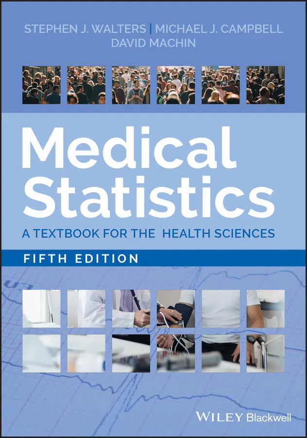
David Machin - Medical Statistics
Здесь есть возможность читать онлайн «David Machin - Medical Statistics» — ознакомительный отрывок электронной книги совершенно бесплатно, а после прочтения отрывка купить полную версию. В некоторых случаях можно слушать аудио, скачать через торрент в формате fb2 и присутствует краткое содержание. Жанр: unrecognised, на английском языке. Описание произведения, (предисловие) а так же отзывы посетителей доступны на портале библиотеки ЛибКат.
- Название:Medical Statistics
- Автор:
- Жанр:
- Год:неизвестен
- ISBN:нет данных
- Рейтинг книги:3 / 5. Голосов: 1
-
Избранное:Добавить в избранное
- Отзывы:
-
Ваша оценка:
Medical Statistics: краткое содержание, описание и аннотация
Предлагаем к чтению аннотацию, описание, краткое содержание или предисловие (зависит от того, что написал сам автор книги «Medical Statistics»). Если вы не нашли необходимую информацию о книге — напишите в комментариях, мы постараемся отыскать её.
Helpful multi-choice exercises are included at the end of each chapter, with answers provided at the end of the book. Each analysis technique is carefully explained and the mathematics kept to minimum. Written in a style suitable for statisticians and clinicians alike, this edition features many real and original examples, taken from the authors' combined many years' experience of designing and analysing clinical trials and teaching statistics.
Students of the health sciences, such as medicine, nursing, dentistry, physiotherapy, occupational therapy, and radiography should find the book useful, with examples relevant to their disciplines. The aim of training courses in medical statistics pertinent to these areas is not to turn the students into medical statisticians but rather to help them interpret the published scientific literature and appreciate how to design studies and analyse data arising from their own projects. However, the reader who is about to design their own study and collect, analyse and report on their own data will benefit from a clearly written book on the subject which provides practical guidance to such issues.
The practical guidance provided by this book will be of use to professionals working in and/or managing clinical trials, in academic, public health, government and industry settings, particularly medical statisticians, clinicians, trial co-ordinators. Its practical approach will appeal to applied statisticians and biomedical researchers, in particular those in the biopharmaceutical industry, medical and public health organisations.
Medical Statistics — читать онлайн ознакомительный отрывок
Ниже представлен текст книги, разбитый по страницам. Система сохранения места последней прочитанной страницы, позволяет с удобством читать онлайн бесплатно книгу «Medical Statistics», без необходимости каждый раз заново искать на чём Вы остановились. Поставьте закладку, и сможете в любой момент перейти на страницу, на которой закончили чтение.
Интервал:
Закладка:
Table 2.6 Calculation of the variance and standard deviation for 16 subjects from the corn size data.
| Corn | Square of | ||||
|---|---|---|---|---|---|
| size | Differences | differences | |||
| Subject | ( mm ) | Mean | from mean | from mean | |
| ( i ) | ( x i) | (  ) ) |
(  ) ) |
(  ) 2 ) 2 |
|
| 1 | 1 | 3.625 | −2.625 | 6.891 | |
| 2 | 2 | 3.625 | −1.625 | 2.641 | |
| 3 | 2 | 3.625 | −1.625 | 2.641 | |
| 4 | 2 | 3.625 | −1.625 | 2.641 | |
| 5 | 2 | 3.625 | −1.625 | 2.641 | |
| 6 | 2 | 3.625 | −1.625 | 2.641 | |
| 7 | 3 | 3.625 | −0.625 | 0.391 | |
| 8 | 3 | 3.625 | −0.625 | 0.391 | |
| 9 | 3 | 3.625 | −0.625 | 0.391 | |
| 10 | 3 | 3.625 | −0.625 | 0.391 | |
| 11 | 4 | 3.625 | 0.375 | 0.141 | |
| 12 | 4 | 3.625 | 0.375 | 0.141 | |
| 13 | 5 | 3.625 | 1.375 | 1.891 | |
| 14 | 6 | 3.625 | 2.375 | 5.641 | |
| 15 | 6 | 3.625 | 2.375 | 5.641 | |
| 16 | 10 | 3.625 | 6.375 | 40.641 | |
| Total | 58 | 0.000 | 75.756 | ||
| n | Mean | df = n−1 | Variance | SD | |
| 16 | 3.625 mm | 15 | 5.050 mm 2 | 2.247 mm |
Why is the Standard Deviation Useful?
From the corn plaster trial data, the mean and standard deviation of the baseline corn size of the 200 trial patients are 3.8 and 1.8 mm respectively (two baseline sizes were missing). It turns out in many situations that about 95% of observations will be within two standard deviations of the mean. This is known as a reference interval or reference range and it is this characteristic of the standard deviation which makes it so useful. It holds for a large number of measurements commonly made in medicine. In particular it holds for data that follow a Normal distribution (see Chapter 4).
For example, the Association for Clinical Biochemistry and Laboratory Medicine gives a number of reference ranges in biochemistry such as for serum potassium of 3.5–5.3 mmol l −1(labtestsonline 2019, https://labtestsonline.org.uk/articles/laboratory‐test‐reference‐ranges). This means in a normal, health population we would expect 19 out of 20 people to have serum potassium levels within these limits. For the corn plaster example, we would expect the majority of corns will be sized between 3.8–1.96 × 1.8 to 3.8 + 1.96 × 1.8 or 0.2 and 7.4 mm. Table 2.7shows that there are 10 patients out of 200 (or 5%) who have a corn size above 7.4 mm and none below 1 mm; thus 95% of the observations in the data lie with two standard deviations of the mean.
Table 2.7 Frequency distribution the size of the corn, in mm, at baseline for 200 patients with corns who were recruited to a randomised control trial of the effectiveness of salicylic acid plasters compared with ‘usual’ scalpel debridement for the treatment of corns
( Source: data from Farndon et al. 2013).
| Size of corn at baseline (mm) | Frequency | Percentage | Cumulative percentage |
|---|---|---|---|
| 1 to <2 | 6 | 3.0 | 3.0 |
| 2 to <3 | 39 | 19.5 | 22.5 |
| 3 to <4 | 52 | 26.0 | 48.5 |
| 4 to <5 | 42 | 21.0 | 69.5 |
| 5 to <6 | 38 | 19.0 | 88.5 |
| 6 to <7 | 10 | 5.0 | 93.5 |
| 7 to <8 | 3 | 1.5 | 95.0 |
| 8 to <9 | 5 | 2.5 | 97.5 |
| 9 to <10 | 1 | 0.5 | 98.0 |
| 10 to <11 | 4 | 2.0 | 100 |
| Total | 200 | 100 |
As we have noted, standard deviation is often abbreviated to SD in the medical literature. Sometimes for emphasis we will denote it by SD( x ), where the bracketed term x is included for a reason to be introduced later.
Means or Medians?
Means and medians convey different impressions of the location of data, and one cannot give a prescription as to which is preferable; often both give useful information. If the distribution is symmetric, then in general the mean is the better summary statistic, and if it is skewed then the median is less influenced by the tails. If the data are skewed, then the median will reflect a ‘typical’ individual better. For example, if in a country median income is £20 000 and mean income is £24 000, most people will relate better to the former number.
It is sometimes stated, incorrectly, that the mean cannot be used with binary, or ordered categorical data but, as we have noted before, if binary data are scored 0/1 then the mean is simply the proportion of 1s. If the data are ordered categorical, then again the data can be scored, say 1, 2, 3, etc. and a mean calculated. This can often give more useful information than a median for such data, but should be used with care, because of the implicit assumption that the change from score 1 to 2, say, has the same meaning (value) as the change from score 2 to 3, and so on.
2.5 Displaying Continuous Data
A picture is worth a thousand words, or numbers, and there is no better way of getting a ‘feel’ for the data than to display them in a figure or graph. The general principle should be to convey as much information as possible in the figure, with the constraint that the reader is not overwhelmed by too much detail.
Dot Plots
The simplest method of conveying as much information as possible is to show all of the data and this can be conveniently carried out using a dot plot. It is also useful for showing the distributions in two or more groups side by side.
Example – Dot Plot – Baseline Corn Size
The data on corn size and treatment group (corn plaster or scalpel) are shown in Figure 2.5as a dot plot. This method of presentation retains the individual subject values and clearly demonstrates any similarities or differences between the groups in a readily appreciated manner. An additional advantage is that any outliers will be detected by such a plot. However, such presentation is not usually practical with large numbers of subjects in each group because the dots will obscure the details of the distribution. Figure 2.5shows that the two randomised groups had similar distributions of corn sizes at baseline.
Читать дальшеИнтервал:
Закладка:
Похожие книги на «Medical Statistics»
Представляем Вашему вниманию похожие книги на «Medical Statistics» списком для выбора. Мы отобрали схожую по названию и смыслу литературу в надежде предоставить читателям больше вариантов отыскать новые, интересные, ещё непрочитанные произведения.


Обсуждение, отзывы о книге «Medical Statistics» и просто собственные мнения читателей. Оставьте ваши комментарии, напишите, что Вы думаете о произведении, его смысле или главных героях. Укажите что конкретно понравилось, а что нет, и почему Вы так считаете.