David Machin - Medical Statistics

With currently available graphics software one can now perform extensive exploration of the data, not only to determine more carefully their structure, but also to find the best means of summary and presentation. This is usually worth considerable effort.

Although graphical presentation is very desirable it should not be overlooked that tabular methods are very important (see Table 2.3). In particular, tables can give more precise numerical information than a graph, such as the number of observations, the mean and some measure of variability of each tabular entry. They often take less space than a graph containing the same information. Standard statistical computer software can be programmed to provide basic summary statistics in tabular form on many variables.

1 Is the number of subjects involved clearly stated?

2 Are appropriate measures of location and variation used in the paper? For example, if the distribution of the data is skewed, then has the median rather the mean been quoted? Is it sensible to quote a standard deviation, or would a range or interquartile range, be better? In general do not use SD for data which have skewed distributions.

3 On graphs, are appropriate axes clearly labelled and scales indicated?

4 Do the titles adequately describe the contents of the tables and graphs?

5 Do the graphs indicate the relevant variability? For example, if the main object of the study is a within‐subject comparison, has the within‐subject variability been illustrated?

6 Does the method of display convey all the relevant information in a study? Can one assess the distribution of the data from the information given?

If the n observations in a sample are arranged in increasing or decreasing order, the median is the middle value. If there are n observations the median is the ½( n + 1)th ordered value. If the number of observations, n , is odd there will be a unique median – the ½( n + 1)th ordered value. If n is even , there is strictly no middle observation, but the median is defined by convention as the mean of the two middle observations – the ½ n th and (½ n + 1)th.

Calculating the median for the foot corn size data, as the number of observations is even ( n = 16), the median is the average of the two middle observations – the ½(16)th and ([½ × 16] + 1)th, i.e. the eighth and ninth ordered values. So the median corn size is (3 + 3)/2 = 3 mm.

Arrange the n observations in increasing or decreasing order. Split the data set into four equal parts –or quartiles using three cut‐points:

1 Lower quartile (25th centile) or the ¼(n + 1)th ordered value;

2 Median(50th centile) or the ½ (n + 1)th ordered value;

3 Upper quartile(75th centile) or the ¾(n + 1)th ordered value.

The interquartile range (IQR) is the upper quartile minus the lower quartile.

It should be noted there is not a single standard convention for calculating the quartiles. When the quartile lies between two observations the simplest option is to take the mean of the two observations. A second option is for the lower and upper quartiles to be the ¼( n + 1)th and ¾( n + 1)th ordered values respectively. A third option is for the lower and upper quartiles to be the ¼ n +½ and ¾ n + ½ ordered values respectively. It is also common to round the ¼ and ¾ to the nearest integer and only use interpolation when this involves calculation of the midpoint of two values. Differences between the results using the different conventions are usually small and unimportant in practice.

To calculate the quartiles for the foot corn size data in Tables 2.4and 2.5, as the number of observations is even ( n = 16), the upper quartile is the ¾( n + 1)th ordered value or ¾ (17)th = 12¾ ordered value. When the quartile lies between two observations the easiest option is to take the mean (there are more complicated methods). The upper quartile ( simple method )is the mean of the 12th and 13th ordered values or (4 + 5)/2 = 4.5 mm. Rounding the 12¾ ordered value to the nearest integer (the 13 thordered value) gives an upper quartile of 5 mm.

A more complicated method for estimating the upper quartile is by interpolation between the 12th and 13th ordered values. The interpolation involves moving ¾ of the way from the 12th ordered value towards the 13th value, i.e. 4 + ¾ (4 to 5) = 4.75 mm (or 4.8 mm when rounding to one decimal place).

The lower quartile is the ¼( n + 1)th ordered value or ¼(17)th = 4¼ ordered value. The lower quartile (simple method) is the mean of the 4th and 5th ordered values or (2 + 2)/2 = 2.0 mm. Rounding the 4¼ ordered value to the nearest integer (the 4 thordered value) gives a lower quartile of 2 mm. A more complicated method for estimating the lower quartile is by interpolation between the fourth and fifth ordered values. The interpolation involves moving ¼ of the way from the fourth ordered value towards the fifth value, i.e. 2 + ¼ (2 to 2) = 2 mm (or 2.0 mm when rounding to 1 decimal place). The IQR estimated by the simple method is 2.0 to 4.5 mm vs 2.0 to 5.0 mm (using the rounding to the nearest integer method) vs 2.0 to 4.8 mm using the more complex interpolation method. As we already mentioned the differences between the results using the different conventions for calculating the quartiles are usually small and unimportant in practice.

Figure 2.11shows the anatomical site of the foot corn by randomised group for 201 patients (Farndon et al. 2013) who were taking part in a randomised controlled trial to investigate the effectiveness of salicylic acid plasters compared with usual scalpel debridement for treatment.

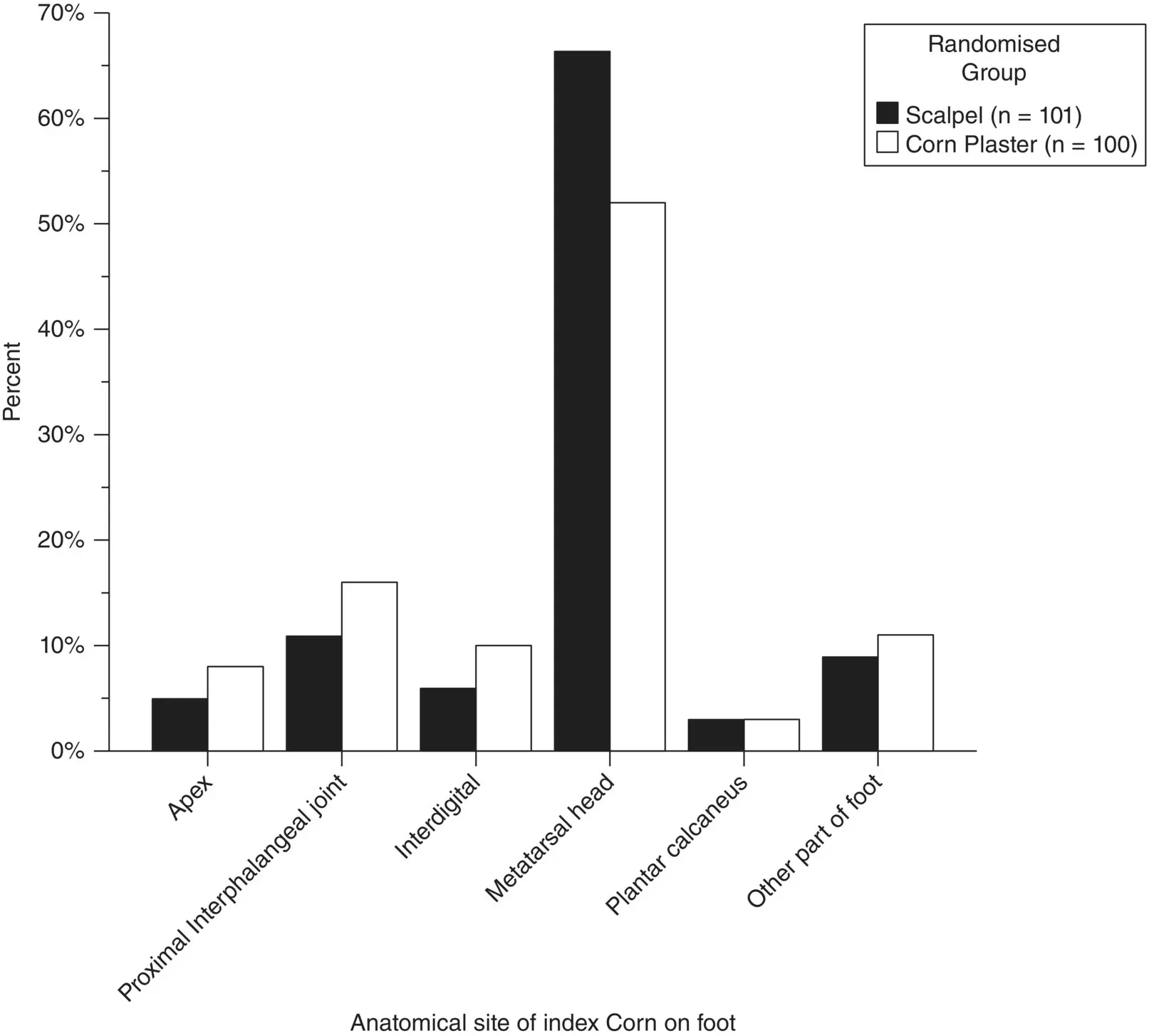
Figure 2.11 Anatomical site of corn on the foot by randomised group for 201 patients with corns

( Source: Farndon et al. 2013).

1 2.1 What type of graph is Figure 2.11?Bar chartPie chartHistogramScatterplotDot plot

2 2.2 What type of data in Figure 2.11is anatomical site of foot corn?DiscreteNominalBinaryOrdinalContinuous

3 2.3 Using the data shown in Figure 2.11which anatomical site of the corn on the foot was the least frequently reported patients in the corn plaster group? The least frequently reported anatomical site of the corn on the foot patients in the corn plaster group was:ApexProximal interphalangeal jointInterdigitalMetatarsal headPlantar calcaneus

4 2.4 Using the data shown in Figure 2.11, approximately how many patients in the scalpel treated group had corn on the proximal interphalangeal joint (middle part of toe on the top)?The approximate number of patients in the scalpel treated group with a corn on the proximal interphalangeal joint was:5811 50100

5 2.5 Using the data shown in Figure 2.11, what approximate percentage of the sample of patients in the corn plaster treated group had a corn on the metatarsal head (ball of the foot at the bottom)?The approximate percentage of patients in the corn plaster treated group who had a corn on the metatarsal head was:20%30%40%50%60%The baseline corn size, in mm, of 10 randomly selected patients from the corn plaster randomised controlled trial (RCT) (Farndon et al. 2013) are given below2 2 2 3 4 4 5 5 7 10