Process Intensification and Integration for Sustainable Design
Здесь есть возможность читать онлайн «Process Intensification and Integration for Sustainable Design» — ознакомительный отрывок электронной книги совершенно бесплатно, а после прочтения отрывка купить полную версию. В некоторых случаях можно слушать аудио, скачать через торрент в формате fb2 и присутствует краткое содержание. Жанр: unrecognised, на английском языке. Описание произведения, (предисловие) а так же отзывы посетителей доступны на портале библиотеки ЛибКат.
- Название:Process Intensification and Integration for Sustainable Design
- Автор:
- Жанр:
- Год:неизвестен
- ISBN:нет данных
- Рейтинг книги:4 / 5. Голосов: 1
-
Избранное:Добавить в избранное
- Отзывы:
-
Ваша оценка:
Process Intensification and Integration for Sustainable Design: краткое содержание, описание и аннотация
Предлагаем к чтению аннотацию, описание, краткое содержание или предисловие (зависит от того, что написал сам автор книги «Process Intensification and Integration for Sustainable Design»). Если вы не нашли необходимую информацию о книге — напишите в комментариях, мы постараемся отыскать её.
Process Intensification and Integration for Sustainable Design
Covers the many advances and changes in process intensification and integration Provides side-by-side discussions of fundamental techniques and recent industrial experiences to guide practitioners in their own processes Presents comprehensive coverage of topics relevant, among others, to the process industry, biorefineries, and plant energy management Offers insightful analysis and integration of reactor and heat exchanger network Looks at optimization of integrated water and multi-regenerator membrane systems involving multi-contaminants
is an ideal book for process engineers, chemical engineers, engineering scientists, engineering consultants, and chemists.
Process Intensification and Integration for Sustainable Design — читать онлайн ознакомительный отрывок
Ниже представлен текст книги, разбитый по страницам. Система сохранения места последней прочитанной страницы, позволяет с удобством читать онлайн бесплатно книгу «Process Intensification and Integration for Sustainable Design», без необходимости каждый раз заново искать на чём Вы остановились. Поставьте закладку, и сможете в любой момент перейти на страницу, на которой закончили чтение.
Интервал:
Закладка:
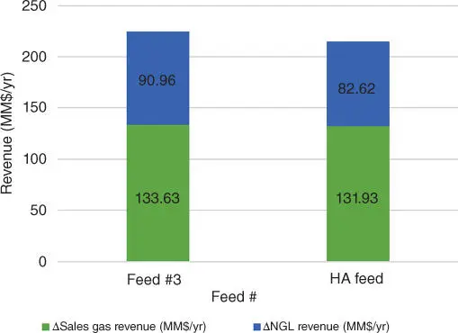
Figure 2.11Revenue for the high acid gas case and base case (MM$/yr).
As shown in Table 2.8, the additional TCI required to treat this stream is not significant, as compared with the additional revenue, and therefore this stream is clearly worth treating (IROI > 10%).
Table 2.8Incremental return on investment for high acid case.
| HA feed | |
| ΔAnnual net profit (MM$/yr) | 11.8 |
| ΔTotal capital investment (MM$/yr) | 6.15 |
| Incremental ROI (%) | 192 |
2.5.4 Safety Index Results
PRI is a relative comparison. The exact values from the calculations are not meaningful, only the relative comparison between different process routes, or in this case different incoming feeds. Only streams where a significant change in composition, pressure, or fluid density occurs were included in the calculation.
One significant weakness of PRI is that is uses the overall average value of each property for all the streams, effectively treating every stream considered as if it has the same flow rate (and thus same potential risk). This leads to misleading results; to give a more truthful picture, the values of each of the four properties used to calculate PRI (mass heating value, fluid density, pressure, and explosiveness) were multiplied by their flow rates as presented in Table 2.9.
Table 2.9Results from modified process route index calculations.
| Feed #1 | Feed #2 | Feed #3 | Feed #4 | Feed #5 | HA feed | |
| Overall | 19.48 | 27.85 | 31.83 | 34.03 | 34.43 | 26.83 |
The lower methane cases are less safe to process. This is because the flows are generally larger in these designs because dehydration is more difficult, and because the fractionation process has higher flow rates due to higher NGL content. Nonetheless there is really not a significant difference in these process designs from a safety perspective. Therefore economic criteria should be the main concern for deciding whether or not to treat streams.
2.5.5 Sensitivity Analysis
One issue of great concern for shale gas producers is price volatility. The price of heating value and of NGLs has fluctuated significantly over the last 15 years [33]. The average and standard deviation for NGL and heating value price data were determined assuming a normal distribution (see Table 2.10) [25].
Table 2.10Maximum, minimum, average, and standard deviation for price data.
| Maximum | Minimum | Average | Standard deviation | |
| Heating value ($/MMBtu) | US$13.42 | US$1.72 | US$4.40 | US$2.22 |
| Ethane ($/gal) | US$1.39 | US$0.14 | US$0.43 | US$0.27 |
| Propane ($/gal) | US$1.89 | US$0.36 | US$0.97 | US$0.37 |
| n ‐Butane ($/gal) | US$2.31 | US$0.49 | US$1.26 | US$0.47 |
A Monte Carlo simulation with 10 000 iterations was performed to find the probability of not being profitable for the base case (when ROI < 10%). Variables were set to be distributed normally in the simulation program. The probability of losing money was about 36%. The average ROI was about 59%; however the standard deviation from the Monte Carlo was approximately 135%. Clearly the shale gas processing business is potentially very profitable, but also very risky. The measured contributions to variance on ROI are shown in Figure 2.12.
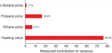
Figure 2.12Measured contributions to variance on ROI for the inputs.
By far the biggest contributor is the heating value, which affects both raw material cost and the sales gas price. This makes sense because methane is the predominant component for this feed (77.78 mol%).
2.5.5.1 Heating Value Cases
Next a few specific cases are considered as shown in Table 2.11. The heating value price affects both the methane and the feedstock price. A higher price for heating value increases both the methane sales prices (which increases potential profitability) and increases the feedstock price (which decreases potential profitability). A sensitivity analysis is used to show which of these counteracting effects is more significant.
Table 2.11Description of Cases 1–3 for sensitivity analysis.
| Case 1 | Case 2 | Case 3 | |
| Heating value | −1 Standard deviation | Average | +1 Standard deviation |
| NGL prices | Average | Average | Average |
The results in Figure 2.13show the process is more profitable at lower heating value prices. This means the methane is being sold for less; however this reduction in revenue is more than offset by the reduction in feedstock cost. A further calculation shows, assuming average NGL prices, the heating value price must be less than US$5.42 per MMBtu to achieve an ROI of more than 10%.
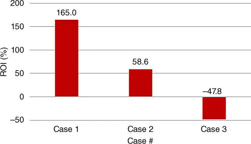
Figure 2.13Results for Cases 1–3 for the sensitivity analysis.
2.5.5.2 NGL Price Cases
Figure 2.14shows NGL prices over time are correlated. Therefore cases where the NGL product prices fluctuated together were considered ( Table 2.12). Since for a normal distribution 99.7% of the values lie within 3 standard deviations of the mean, ±3 standard deviations were chosen for the cases (prices were not allowed to be negative). Since the main question is whether the process will be profitable or not, only the deviations in the direction that would make the process less profitable were examined.
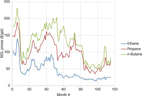
Figure 2.14Price of products over time [34].
Table 2.12Description of cases for sensitivity analysis.
| Case 4 | Case 5 | Case 6 | |
| Heating value | Average | Average | Average |
| NGL prices | −1 Standard deviation | −2 Standard deviation | −3 Standard deviation |
As can be seen in Figure 2.15, for even a drop of 1 standard deviation in NGL prices, the ROI value will become negative. This occurs because the standard deviations of the product prices are very high. An additional calculation shows that to achieve an ROI of more than 10%, product prices cannot drop more than 16.5%, assuming an average heating value price.
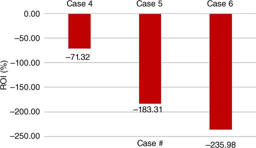
Figure 2.15Results for Cases 4–6 for the sensitivity analysis.
2.6 Conclusions
A methodology was developed for process design under uncertainty for a shale gas treatment plant. An integrated approach of process simulation, design under uncertainty, techno‐economic analysis, and safety assessment was used to determine the optimal design of the gas treatment plant. A number of feeds with varying inlet compositions were examined to represent the uncertain compositions of shale gas. A case study was carried out for data from the Barnett Shale Play.
Читать дальшеИнтервал:
Закладка:
Похожие книги на «Process Intensification and Integration for Sustainable Design»
Представляем Вашему вниманию похожие книги на «Process Intensification and Integration for Sustainable Design» списком для выбора. Мы отобрали схожую по названию и смыслу литературу в надежде предоставить читателям больше вариантов отыскать новые, интересные, ещё непрочитанные произведения.


Обсуждение, отзывы о книге «Process Intensification and Integration for Sustainable Design» и просто собственные мнения читателей. Оставьте ваши комментарии, напишите, что Вы думаете о произведении, его смысле или главных героях. Укажите что конкретно понравилось, а что нет, и почему Вы так считаете.