Process Intensification and Integration for Sustainable Design
Здесь есть возможность читать онлайн «Process Intensification and Integration for Sustainable Design» — ознакомительный отрывок электронной книги совершенно бесплатно, а после прочтения отрывка купить полную версию. В некоторых случаях можно слушать аудио, скачать через торрент в формате fb2 и присутствует краткое содержание. Жанр: unrecognised, на английском языке. Описание произведения, (предисловие) а так же отзывы посетителей доступны на портале библиотеки ЛибКат.
- Название:Process Intensification and Integration for Sustainable Design
- Автор:
- Жанр:
- Год:неизвестен
- ISBN:нет данных
- Рейтинг книги:4 / 5. Голосов: 1
-
Избранное:Добавить в избранное
- Отзывы:
-
Ваша оценка:
Process Intensification and Integration for Sustainable Design: краткое содержание, описание и аннотация
Предлагаем к чтению аннотацию, описание, краткое содержание или предисловие (зависит от того, что написал сам автор книги «Process Intensification and Integration for Sustainable Design»). Если вы не нашли необходимую информацию о книге — напишите в комментариях, мы постараемся отыскать её.
Process Intensification and Integration for Sustainable Design
Covers the many advances and changes in process intensification and integration Provides side-by-side discussions of fundamental techniques and recent industrial experiences to guide practitioners in their own processes Presents comprehensive coverage of topics relevant, among others, to the process industry, biorefineries, and plant energy management Offers insightful analysis and integration of reactor and heat exchanger network Looks at optimization of integrated water and multi-regenerator membrane systems involving multi-contaminants
is an ideal book for process engineers, chemical engineers, engineering scientists, engineering consultants, and chemists.
Process Intensification and Integration for Sustainable Design — читать онлайн ознакомительный отрывок
Ниже представлен текст книги, разбитый по страницам. Система сохранения места последней прочитанной страницы, позволяет с удобством читать онлайн бесплатно книгу «Process Intensification and Integration for Sustainable Design», без необходимости каждый раз заново искать на чём Вы остановились. Поставьте закладку, и сможете в любой момент перейти на страницу, на которой закончили чтение.
Интервал:
Закладка:
2.4 Case Study
To illustrate the applicability of the proposed approach, a case study is solved based on representative data for the Barnett Shale Play in Texas. The key objectives of the case study include:
Design of a base case and several additional process designs for different feed compositions
Economic evaluations of the proposed designs
Process safety evaluation of the proposed designs
Sensitivity analysis where product and feedstock prices are varied based on standard deviations from historical price data
To streamline the study, the following assumptions are made:
Average flow rate, temperature, and pressure: Although the flow rate, temperature, and pressure of shale gas coming out of the well can vary significantly, it was assumed that wellhead gas is sent to a centralized processing facility where these values on average would be relatively constant, and only composition would vary. Additionally it is common for gas to be saturated with water because water is sent down the well to maintain well pressure. It is not uncommon for there to also be free water in the incoming gas stream; however this is easily removed using a knockout drum on the front end of the process at minimal cost.
Inlet feeds enter the processing plant at a standard vapor volumetric flow of 150 million standard cubic feet per day (MMSCFD), 100 °F, and 1000 psig. The Peng–Robinson equation of state was used in the process simulation model.
The gas feedstock is saturated with water.
2.4.1 Data
First, compositional data was obtained for the Barnett Shale region (located in the Dallas, TX, area) [3]. Next, minor components such as nitrogen, oxygen, and hydrogen were removed from the data sets so that only the major components (CO 2and the hydrocarbons) were considered. The compositional data sets were classified into different types. This was done based on the methane composition in each data set. There were five types of data sets as shown in Table 2.1. Table 2.1also shows the probability of each feed type as determined from the literature data [3].
Table 2.1Feed types as determined by methane composition.
| Feed type | Methane composition (mol%) | Probability of feed type (%) |
| 1 | >87 | 7.50 |
| 2 | 81–87 | 28.33 |
| 3 | 75–81 | 28.33 |
| 4 | 69–75 | 28.33 |
| 5 | <69 | 7.50 |
Next, one case from each feed type was selected from among the data sets. The case chosen for each feed type was a case found near the middle of the distribution. A total of five cases were selected (see Table 2.2). From among these cases, the base case was selected as type 3 case since it falls nearest to the middle of the distribution and is representative of the most commonly found composition in this region.
Table 2.2Selected cases.
| Composition (mol%) | Feed #1 | Feed #2 | Feed #3 | Feed #4 | Feed #5 |
| Methane | 94.11 | 83.62 | 77.78 | 71.94 | 56.34 |
| Ethane | 2.59 | 7.54 | 9.42 | 11.55 | 16.13 |
| Propane | 0.02 | 4.68 | 7.26 | 9.60 | 16.06 |
| n ‐Butane | 0.25 | 2.11 | 2.65 | 3.15 | 4.96 |
| i ‐Butane | 0.26 | 1.08 | 1.27 | 1.61 | 2.62 |
| n ‐Pentane | 0.02 | 0.30 | 0.60 | 0.82 | 1.60 |
| i ‐Pentane | 0.03 | 0.30 | 0.53 | 0.76 | 1.44 |
| Neopentane | 0.00 | 0.00 | 0.00 | 0.02 | 0.04 |
| Carbon dioxide | 2.71 | 0.38 | 0.49 | 0.56 | 0.81 |
Finally one additional case is considered. As mentioned in the introduction, sulfur species, predominately hydrogen sulfide, may also be found in shale gas [6]. The goal of considering this case is to determine if the additional processing needed for a gas with a high acid (HA) loading would significantly affect the economics of treating such a stream. This inlet composition of this case was chosen such that the methane and NGL content would be similar to that of the base case (Feed #3) ( Table 2.3).
Table 2.3High acid (HA) gas feed composition.
| Composition (mol%) | HA feed |
| Methane | 74.35 |
| Ethane | 9.00 |
| Propane | 6.94 |
| n ‐Butane | 2.54 |
| i ‐Butane | 1.22 |
| n ‐Pentane | 0.57 |
| i ‐Pentane | 0.51 |
| Neopentane | 0.00 |
| Carbon dioxide | 4.78 |
| Hydrogen sulfide | 0.10 |
2.4.2 Process Simulations and Economic Evaluation
Process simulation was performed to meet the required specifications (sales gas gross heating value of 950–1150 Btu/SCF [British thermal unit/standard cubic feet], 1000 psig, and CO 2content of 2–3 mol% maximum, 0.3 g H 2S/100 SCF gas) [22,23], and process designs were developed for each feed. ProMax simulation software [24] was used to simulate this process.
The simulation results were then used to size process equipment, develop mass and energy balances, and determine operating conditions and utility consumption of process equipment. Aspen process economic analyzer [25] was used to estimate the equipment purchase costs. The Hand factor was utilized to account for installation and other costs. The fixed capital investment (FCI) for each processing unit was then estimated [26].
(2.1) 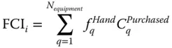
where FCI i, fixed capital investment for a given processing unit;  , Hand factor for equipment q ; and
  , the purchased cost of equipment q .
Table 2.4shows the values and assumptions used to estimate the variable costs (raw material costs were considered separately):
Table 2.4Parameters used for the techno‐economic analysis.
| Parameter | Values | Units | References |
| Variable cost parameters | |||
| TEG price | 0.93 | $/lb | [27] |
| Refrigerant price | 13.11 | $/GJ | [28] |
| Electricity price | 0.049 | $/kWh | [29] |
| Fuel price | 2.98 | $/MSCF | [30] |
| Plant operator rate | 32.74 | $/h | [31] |
| Plant supervisor rate | 68.13 | $/h | [32] |
| Maintenance | 5 | % of FCI | [25] |
| Operating charges | 25 | % of operating labor cost | [25] |
| Plant overhead | 50 | % of operating labor + maintenance cost | [25] |
| General administrative | 8 | % of all other operating costs | [25] |
| Stream factor | 0.96 | — | — |
The only additional equations used were those to estimate the number of workers based on the number of processing steps [28]:
Читать дальшеИнтервал:
Закладка:
Похожие книги на «Process Intensification and Integration for Sustainable Design»
Представляем Вашему вниманию похожие книги на «Process Intensification and Integration for Sustainable Design» списком для выбора. Мы отобрали схожую по названию и смыслу литературу в надежде предоставить читателям больше вариантов отыскать новые, интересные, ещё непрочитанные произведения.


Обсуждение, отзывы о книге «Process Intensification and Integration for Sustainable Design» и просто собственные мнения читателей. Оставьте ваши комментарии, напишите, что Вы думаете о произведении, его смысле или главных героях. Укажите что конкретно понравилось, а что нет, и почему Вы так считаете.