Process Intensification and Integration for Sustainable Design
Здесь есть возможность читать онлайн «Process Intensification and Integration for Sustainable Design» — ознакомительный отрывок электронной книги совершенно бесплатно, а после прочтения отрывка купить полную версию. В некоторых случаях можно слушать аудио, скачать через торрент в формате fb2 и присутствует краткое содержание. Жанр: unrecognised, на английском языке. Описание произведения, (предисловие) а так же отзывы посетителей доступны на портале библиотеки ЛибКат.
- Название:Process Intensification and Integration for Sustainable Design
- Автор:
- Жанр:
- Год:неизвестен
- ISBN:нет данных
- Рейтинг книги:4 / 5. Голосов: 1
-
Избранное:Добавить в избранное
- Отзывы:
-
Ваша оценка:
Process Intensification and Integration for Sustainable Design: краткое содержание, описание и аннотация
Предлагаем к чтению аннотацию, описание, краткое содержание или предисловие (зависит от того, что написал сам автор книги «Process Intensification and Integration for Sustainable Design»). Если вы не нашли необходимую информацию о книге — напишите в комментариях, мы постараемся отыскать её.
Process Intensification and Integration for Sustainable Design
Covers the many advances and changes in process intensification and integration Provides side-by-side discussions of fundamental techniques and recent industrial experiences to guide practitioners in their own processes Presents comprehensive coverage of topics relevant, among others, to the process industry, biorefineries, and plant energy management Offers insightful analysis and integration of reactor and heat exchanger network Looks at optimization of integrated water and multi-regenerator membrane systems involving multi-contaminants
is an ideal book for process engineers, chemical engineers, engineering scientists, engineering consultants, and chemists.
Process Intensification and Integration for Sustainable Design — читать онлайн ознакомительный отрывок
Ниже представлен текст книги, разбитый по страницам. Система сохранения места последней прочитанной страницы, позволяет с удобством читать онлайн бесплатно книгу «Process Intensification and Integration for Sustainable Design», без необходимости каждый раз заново искать на чём Вы остановились. Поставьте закладку, и сможете в любой момент перейти на страницу, на которой закончили чтение.
Интервал:
Закладка:
(2.2) 
where N np, the number of non‐particulate processing steps, which is related with the number of operators per shift ( N OL), given as in Eq. (2.3):
(2.3) 
where P , the number of processing steps where particulate solids are handled.
2.4.2.1 Changes in Fixed and Variable Costs
Additional cases were fed through the base case process design, and any needed modifications were made to meet product specifications. Therefore, fixed and variable costs were first estimated as before, and then only the change in each of these costs was used in the subsequent calculations. For fixed costs, the change was only used in cases where the costs were higher, since the need for smaller equipment does not result in any savings for an existing plant.
2.4.2.2 Revenue
Table 2.5shows the price of each component [33]:
Table 2.5Price of different commodities.
| Commodity | Units | Base case |
| Heat valuea | $/MMBtu | 2.98 |
| Ethane | $/gal | 0.262 |
| Propane | $/gal | 0.632 |
| n ‐Butane | $/gal | 0.691 |
aMethane and wellhead gas are priced in terms of their heat value ($/MMBtu).
2.4.2.3 Economic Calculations
The next step was to calculate the return on investment (ROI) [26]:
(2.4) 
where TCI, total capital investment.
First, the quantities in Eqs. must be calculated.
(2.5) 
where FCI, total fixed capital investment:
(2.6) 
where WCI, working capital investment (assumed to be 15% of FCI):
(2.7) 
where AFC, annualized fixed cost (depreciation); FCI S, the salvage value of the FCI (assumed to be 10% of FCI); and N , plant lifetime (assumed to be 10 years):
(2.8) 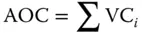
where AOC, annual operating cost; VC i, total variable cost for each process unit:
(2.9) 
where TAC, total annualized cost:
(2.10) 
(2.11) 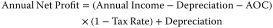
where the tax rate is assumed to be 30%.
For the other cases, the calculations are similar, except instead of fixed and variable costs only the additional costs were determined. This is done because we are considering only the additional costs for processing a new composition. Similarly instead of ROI, incremental return on investment (IROI) is calculated instead:
(2.12) 
where ΔTCI, the change in total capital investment for a given additional case.
Finally, the total ROI can be determined for treating multiple feeds from the following:
(2.13) 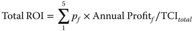
where p , probability or likelihood of obtaining a particular feed, and the subscript f denotes feed.
2.4.3 Safety Index Calculations
A modified version of the PRI was used to evaluate each case in order to incorporate safety considerations into the design process. These calculations were done following the method of Leong and Shariff [18], but the flow rate of each stream was incorporated as follows:
(2.14) 
where  mass flow rate (kg/h); HV m, average mass heating value (kJ/kg); ρ , average fluid density (kg/m 3); P , average pressure (bar); and ΔFL mix, average explosiveness (%), where the explosiveness for each stream is given as the difference between UFL mixand LFL mix:
(2.15) 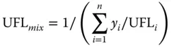
(2.16) 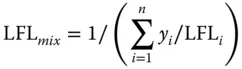
2.5 Discussion
First the process simulation for the six cases is discussed. Specifically the dehydration, the turboexpander, and the fractionation train processes are discussed for all cases. Additionally acid gas removal is considered for the high acid gas case. Acid gas removal is not needed for Feeds #1–5 as acid gas levels (CO 2and H 2S) already meet specifications. Free water removal is not needed, as it is assumed only bound water is present (see Section 2.4).
2.5.1 Process Simulations
2.5.1.1 Dehydration Process
For all five cases, the first unit operation of the gas treatment process is dehydration. The typical dehydration process used in natural gas processing is glycol dehydration, with the flowsheet shown in Figure 2.3. As mentioned previously, the goal of the glycol dehydration process is to remove thermodynamically bound water from the gas to permissible levels. Triethylene glycol (TEG) is the most commonly used solvent in industry for water removal. This process contains two loops, i.e. the contactor loop (where wet gas is contacted with TEG to remove water) and the regenerator loop (where water is removed from TEG in order to recycle the TEG back to the contactor).
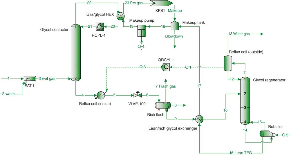
Figure 2.3Glycol dehydration process.
Читать дальшеИнтервал:
Закладка:
Похожие книги на «Process Intensification and Integration for Sustainable Design»
Представляем Вашему вниманию похожие книги на «Process Intensification and Integration for Sustainable Design» списком для выбора. Мы отобрали схожую по названию и смыслу литературу в надежде предоставить читателям больше вариантов отыскать новые, интересные, ещё непрочитанные произведения.


Обсуждение, отзывы о книге «Process Intensification and Integration for Sustainable Design» и просто собственные мнения читателей. Оставьте ваши комментарии, напишите, что Вы думаете о произведении, его смысле или главных героях. Укажите что конкретно понравилось, а что нет, и почему Вы так считаете.