Robert Bartoszynski - Probability and Statistical Inference

Since outcomes can be specified in various ways (as illustrated by Examples 1.1and 1.3), it follows that the same experiment can be described in terms of different sample spaces . The choice of a sample space depends on the goal of description. Moreover, certain sample spaces for the same experiment lead to easier and simpler analysis. The choice of a “better” sample space requires some skill, which is usually gained through experience. The following two examples illustrate this point.

Let the experiment consist of recording the lifetime of a piece of equipment, say a light bulb. An outcome here is the time until the bulb burns out. An outcome typically will be represented by a number ( if the bulb is not working at the start), and therefore is the nonnegative part of the real axis. In practice, is measured with some precision (in hours, days, etc.), so one might instead take . Which of these choices is better depends on the type of subsequent analysis.

Two persons enter a cafeteria and sit at a square table, with one chair on each of its sides. Suppose we are interested in the event “they sit at a corner” (as opposed to sitting across from one another). To construct the sample space, we let A and B denote the two persons, and then take as the set of outcomes represented by 12 ideograms in Figure 1.1. One could argue, however, that such a sample space is unnecessarily large. If we are interested only in the event “they sit at a corner,” then there is no need to label the persons as A and B. Accordingly, the sample space may be reduced to the set of six outcomes depicted in Figure 1.2. But even this sample space can be simplified. Indeed, one could use the rotational symmetry of the table and argue that once the first person selects a chair (it does not matter which one), then the sample space consists of just three chairs remaining for the second person (see Figure 1.3).

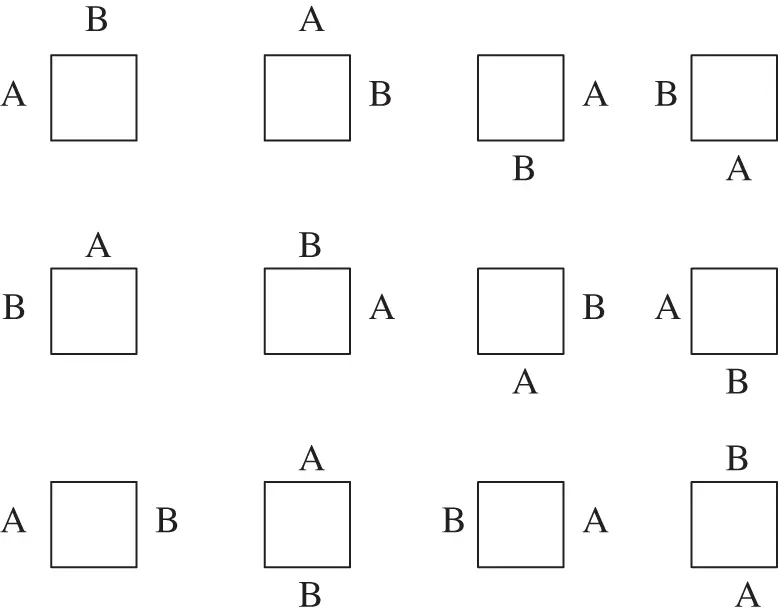
Figure 1.1Possible seatings of persons A and B at a square table.

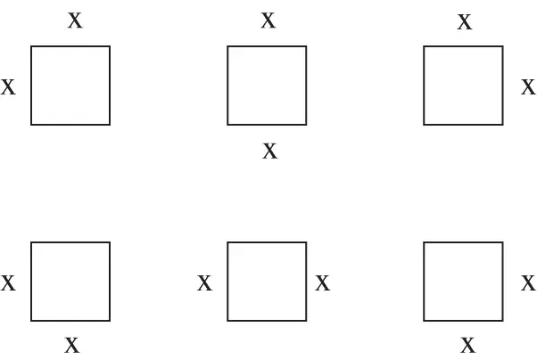
Figure 1.2Possible seatings of any two persons at a square table.

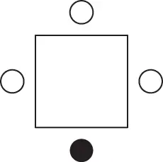
Figure 1.3Possible seatings of one person if the place of the other person is fixed.

Sample spaces can be classified according to the number of sample points they contain. Finite sample spaces contain finitely many outcomes, and elements of infinitely countable sample spaces can be arranged into an infinite sequence; other sample spaces are called uncountable .

The next concept to be introduced is that of an event . Intuitively, an event is anything about which we can tell whether or not it has occurred, as soon as we know the outcome of the experiment. This leads to the following definition:

Definition 1.2.2An event is a subset of the sample space .

In Example 1.1an event such as “the sum equals 7” containing six outcomes and is a subset of the sample space . In Example 1.3, the same event consists of one outcome, 7.

When an experiment is performed, we observe its outcome. In the interpretation developed in this chapter, this means that we observe a point chosen randomly from the sample space. If this point belongs to the subset representing the event , we say that the event A has occurred .

We will let events be denoted either by letters , possibly with identifiers, such as or by more descriptive means, such as and , where and are some numerical attributes of the sample points (formally: random variables, to be discussed in Chapter 5). Events can also be described through verbal phrases, such as “two heads in a row occur before the third tail” in the experiment of repeated tosses of a coin.

In all cases considered thus far, we assumed that an outcome (a point in the sample space) can be observed . To put it more precisely, all sample spaces considered so far were constructed in such a way that their points were observable. Thus, for any event , we were always able to tell whether it occurred or not.