Robert Bartoszynski - Probability and Statistical Inference

The following theorem is an immediate consequence of Theorem 3.3.3applied to and , respectively.

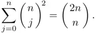
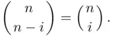
Theorem 3.3.4 The binomial coefficients satisfy the identities

(3.17)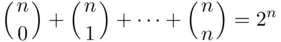

and

(3.18)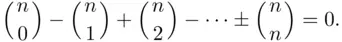

We also have the following theorem:

Theorem 3.3.5 For every and every

(3.19)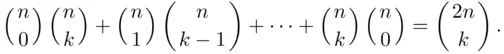

Proof : Consider the product . Expanding the right‐hand side, we obtain

(3.20)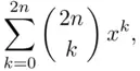

while the left‐hand side equals

(3.21)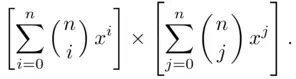

For , comparison of the coefficients of in ( 3.20) and ( 3.21) gives ( 3.19).

As a consequence of ( 3.19), we obtain a corollary:

Proof : Take in ( 3.19) and use the fact that

Below we present some examples of the use of binomial coefficient in solving various probability problems, some with a long history.

Let us consider a selection without replacement from a finite set containing two categories of objects. If balls are to be selected from an urn containing red and blue balls, one might want to know the probability that there will be exactly red balls chosen.

We apply here the “classical” definition of probability. The choice of objects without replacement is the same as choosing a subset of objects from the set of total of objects. This can be done in different ways. Since we must have red balls, this choice can be made in ways. Similarly, blue balls can be selected in ways. As each choice of red balls can be combined with each of the choices of blue balls then, by Theorem 3.2.2, the total number of choices is the product 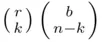and

(3.22)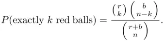

The next example shows an interesting application of formula ( 3.22).

Consider the problem of estimating the number of fish in a lake (the method described below is also used to estimate the sizes of bird or wildlife populations). The lake contains an unknown number of fish. To estimate , we first catch fish, label them, and release them back into the lake. We assume here that labeling does not harm fish in any way, that the labeled fish mix with unlabeled ones in a random manner, and that remains constant (in practice, these assumptions may be debatable). We now catch fish, and observe the number, say , of labeled ones among them. The values and are, at least partially, under the control of the experimenter. The unknown parameter is , while is the value occurring at random, and providing the key to estimating . Let us compute the probability of observing labeled fish in the second catch if there are fish in the lake. We may interpret fish as balls in an urn, with labeled and unlabeled fish taking on the roles of red and blue balls. Formula ( 3.22) gives