Matthew B. Hamilton - Population Genetics

(2.28)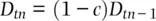

Since gametic disequilibrium decays by a factor of 1 − c each generation,

(2.29)

We can predict the amount of gametic disequilibrium over time by using the amount of disequilibrium initially present ( D t0) and multiplying it by (1 − c ) raised to the power of the number of generations that have elapsed:

(2.30)

Figure 2.19shows the decay of gametic disequilibrium over time using Eq. 2.30. Initially, there are only coupling gametes in the population and no repulsion gametes, giving a maximum amount of gametic disequilibrium. As c increases, the approach to gametic equilibrium ( D = 0) is more rapid. Eq. 2.30and Figure 2.20both assume that there are no other processes acting to counter the mixing effect of recombination. Therefore, the steady‐state will always be equal frequencies of all gametes ( D = 0), with the recombination rate determining how rapidly gametic equilibrium is attained.

A hypothesis test that the observed level of gametic disequilibrium is significantly different than expected under random segregation can be carried out with:

(2.31)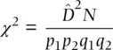

where N is the total sample size of gametes, is a gametic disequilibrium estimate, and p and q are the allele frequencies at two diallelic loci. The χ 2value has 1 degree of freedom and can be compared with the critical value found in Table 2.5.

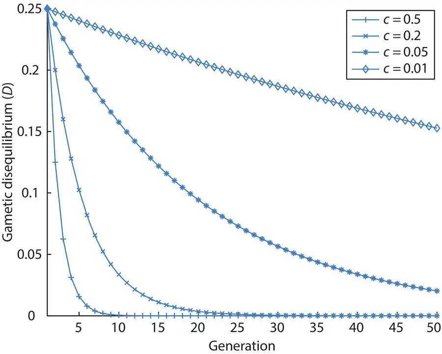
Figure 2.19 The decay of gametic disequilibrium ( D ) over time for four recombination rates. Initially, there are only coupling ( P 11= P 22= ½) and no repulsion gametes ( P 12= P 21= 0). Gametic disequilibrium decays as a function of time and the recombination rate ( D t = n= D t = 0[1− c ] n) assuming a single large population, random mating and no counteracting genetic processes. If all gametes were initially repulsion, gametic disequilibrium would initially equal −0.25 and decay to zero in an identical fashion.

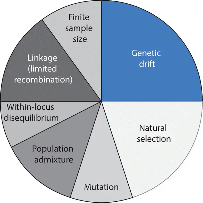
Figure 2.20 A hypothetical partitioning of the contributions to the total population gametic disequilibrium ( D ) in a population caused by numerous population genetic processes. The finite sample of gametes or genotypes used to measure D can itself contribute to the disequilibrium observed, as can departure from Hardy–Weinberg expected genotype frequencies at single loci or within‐locus disequilibrium. The fractions of the total gametic disequilibrium attributable to each cause will vary depending on history of a population and the relative strengths of the multiple processes acting in a population.

One potential drawback of D in Eq. 2.27is that its maximum value depends on the allele frequencies in the population. This can make interpreting an estimate of D or comparing estimates of D from different populations problematic. For example, it is possible that two populations have very strong association among alleles within gametes (e.g. no repulsion gametes), but the two populations differ in allele frequency so that the maximum value of D in each population is also different. If all alleles are not at equal frequencies in a population, then the frequencies of the two coupling or the two repulsion gametes are also not equal. When D < 0, D maxis the value of − p 1 q 1or − p 2 q 2that is closer to zero, whereas when D > 0, D maxis the value of p 1 q 2or p 2 q 1that is closer to zero.

A way to avoid these problems is to express D as the percentage of its largest value:

(2.32)

This gives a measure of gametic disequilibrium that is normalized by the maximum or minimum value D can assume given population allele frequencies. Even though a given value of D may seem small in the absolute, it may be large relative to D maxgiven the population allele frequencies. A related and more commonly employed measure expresses disequilibrium between two loci as a correlation:

(2.33)

where ρ (pronounced “roe”) takes the familiar and more easily interpreted range of −1 to +1 (the disequilibrium correlation is sometimes given as ρ 2with 0 ≤ ρ 2≤ 1) (Lewontin 1988). Analogous to the fixation index, the two locus disequilibrium correlation can be understood as a measure of the correlation between the states of the two alleles found together in a two locus haplotypes. When ρ = 0 there is no correlation between the alleles at two loci that are found paired in gametes or on the same chromosome – the allelic states are independent as expected under Mendel's second law. If ρ > 0 there is a positive correlation such that if one of the alleles at one locus is an A, for example, then the allele at the second locus will have a correlated state and might often be a B allele. When ρ < 0 there is a negative correlation between the states of two alleles in a haplotype, such as if A is infrequently paired with B.

Thus far, we have approached gametic disequilibrium by focusing on the frequency of four gamete haplotypes. A helpful complement is to consider the gametes made by all possible two locus genotypes as shown in Table 2.12. This table is somewhat like the table of parental matings and their offspring genotype frequencies we made to prove Hardy–Weinberg for one locus, except Table 2.12predicts the frequencies of gametes that will make up the next generation rather than genotype frequencies in the next generation. Most genotypes produce recombinant gametes that are identical to non‐recombinant gametes (e.g. the A 1B 1/A 1B 2genotype produces A 1B 1and A 1B 2coupling gametes and A 1B 1and A 1B 2repulsion gametes). Only two genotypes – both types of double heterozygotes – will produce recombinant gametes that are different than parental haplotypes. These are the only two places where c enters into the expressions for expected gamete frequencies because recombination does not change the gametes produced by the other eight two locus genotypes.

Table 2.12 Expected frequencies of gametes for two diallelic loci in a randomly mating population with a recombination rate between the two loci of c . The first eight genotypes have non‐recombinant and recombinant gametes that are identical. The last two genotypes produce novel recombinant gametes, requiring inclusion of the recombination rate to predict gamete frequencies. Summing down each column of the table gives the total frequency of each gamete in the next generation.