Douglas C. Montgomery - Introduction to Linear Regression Analysis
Здесь есть возможность читать онлайн «Douglas C. Montgomery - Introduction to Linear Regression Analysis» — ознакомительный отрывок электронной книги совершенно бесплатно, а после прочтения отрывка купить полную версию. В некоторых случаях можно слушать аудио, скачать через торрент в формате fb2 и присутствует краткое содержание. Жанр: unrecognised, на английском языке. Описание произведения, (предисловие) а так же отзывы посетителей доступны на портале библиотеки ЛибКат.
- Название:Introduction to Linear Regression Analysis
- Автор:
- Жанр:
- Год:неизвестен
- ISBN:нет данных
- Рейтинг книги:4 / 5. Голосов: 1
-
Избранное:Добавить в избранное
- Отзывы:
-
Ваша оценка:
Introduction to Linear Regression Analysis: краткое содержание, описание и аннотация
Предлагаем к чтению аннотацию, описание, краткое содержание или предисловие (зависит от того, что написал сам автор книги «Introduction to Linear Regression Analysis»). Если вы не нашли необходимую информацию о книге — напишите в комментариях, мы постараемся отыскать её.
New exercises and data sets New material on generalized regression techniques The inclusion of JMP software in key areas Carefully condensing the text where possible
skillfully blends theory and application in both the conventional and less common uses of regression analysis in today's cutting-edge scientific research. The text equips readers to understand the basic principles needed to apply regression model-building techniques in various fields of study, including engineering, management, and the health sciences.
Introduction to Linear Regression Analysis — читать онлайн ознакомительный отрывок
Ниже представлен текст книги, разбитый по страницам. Система сохранения места последней прочитанной страницы, позволяет с удобством читать онлайн бесплатно книгу «Introduction to Linear Regression Analysis», без необходимости каждый раз заново искать на чём Вы остановились. Поставьте закладку, и сможете в любой момент перейти на страницу, на которой закончили чтение.
Интервал:
Закладка:

These expected mean squares indicate that if the observed value of F 0is large, then it is likely that the slope β 1≠ 0. Appendix C.3also shows that if β 1≠ 0, then F 0follows a noncentral F distribution with 1 and n − 2 degrees of freedom and a non-centralityparameter of

This noncentrality parameter also indicates that the observed value of F 0should be large if β 1≠ 0. Therefore, to test the hypothesis H 0: β 1= 0, compute the test statistic F 0and reject H 0if

The test procedure is summarized in Table 2.4.
TABLE 2.4 Analysis of Variance for Testing Significance of Regression
| Source of Variation | Sum of Squares | Degrees of Freedom | Mean Square | F 0 |
| Regression |  |
1 | MS R | MS R/ MS Res |
| Residual | 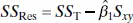 |
n − 2 | MS Res | |
| Total | SS T | n − 1 |
Example 2.4 The Rocket Propellant Data
We will test for significance of regression in the model developed in Example 2.1for the rocket propellant data. The fitted model is 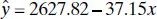 , SS T= 1,693,737.60, and Sxy = −41,112.65. The regression sum of squares is computed from Eq. (2.34)as

The analysis of variance is summarized in Table 2.5. The computed value of F 0is 165.21, and from Table A.4, F 0.01,1,18= 8.29. The P value for this test is 1.66 × 10 −10. Consequently, we reject H 0: β 1= 0.
The Minitab output in Table 2.3 also presents the analysis-of-variance test significance of regression. Comparing Tables 2.3 and 2.5, we note that there are some slight differences between the manual calculations and those performed by computer for the sums of squares. This is due to rounding the manual calculations to two decimal places. The computed values of the test statistics essentially agree.
More About the t Test
We noted in Section 2.3.2that the t statistic
(2.37) 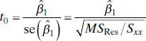
could be used for testing for significance of regression. However, note that on squaring both sides of Eq. (2.37), we obtain
(2.38) 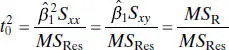
Thus,  in Eq. (2.38)is identical to F 0of the analysis-of-variance approach in Eq. (2.36). For example; in the rocket propellant example t 0= −12.5, so
  . In general, the square of a t random variable with f degrees of freedom is an F random variable with one and f degrees of freedom in the numerator and denominator, respectively. Although the t test for H 0: β 1= 0 is equivalent to the F test in simple linear regression, the t test is somewhat more adaptable, as it could be used for one-sided alternative hypotheses (either H 1: β 1< 0 or H 1: β 1> 0), while the F test considers only the two-sided alternative. Regression computer programs routinely produce both the analysis of variance in Table 2.4 and the t statistic. Refer to the Minitab output in Table 2.3.
TABLE 2.5 Analysis-of-Variance Table for the Rocket Propellant Regression Model
| Source of Variation | Sum of Squares | Degrees of Freedom | Mean Square | F 0 | P value |
| Regression | 1,527,334.95 | 1 | 1,527,334.95 | 165.21 | 1.66 × 10 −10 |
| Residual | 166,402.65 | 18 | 9,244.59 | ||
| Total | 1,693,737.60 | 19 |
The real usefulness of the analysis of variance is in multiple regression models. We discuss multiple regression in the next chapter.
Finally, remember that deciding that β 1= 0 is a very important conclusion that is only aidedby the t or F test. The inability to show that the slope is not statistically different from zero may not necessarily mean that y and x are unrelated. It may mean that our ability to detect this relationship has been obscured by the variance of the measurement process or that the range of values of x is inappropriate. A great deal of nonstatistical evidence and knowledge of the subject matter in the field is required to conclude that β 1= 0.
2.4 INTERVAL ESTIMATION IN SIMPLE LINEAR REGRESSION
In this section we consider confidence interval estimation of the regression model parameters. We also discuss interval estimation of the mean response E ( y ) for given values of x . The normality assumptions introduced in Section 2.3continue to apply.
2.4.1 Confidence Intervals on β 0, β 1, and σ 2
In addition to point estimates of β 0, β 1, and σ 2, we may also obtain confidence interval estimates of these parameters. The width of these confidence intervals is a measure of the overall quality of the regression line. If the errors are normally and independently distributed, then the sampling distribution of both 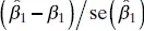 and
and 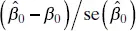 is t with n − 2 degrees of freedom. Therefore, a 100(1 − α ) percent confidence interval (CI) on the slope β 1is given by
Интервал:
Закладка:
Похожие книги на «Introduction to Linear Regression Analysis»
Представляем Вашему вниманию похожие книги на «Introduction to Linear Regression Analysis» списком для выбора. Мы отобрали схожую по названию и смыслу литературу в надежде предоставить читателям больше вариантов отыскать новые, интересные, ещё непрочитанные произведения.


Обсуждение, отзывы о книге «Introduction to Linear Regression Analysis» и просто собственные мнения читателей. Оставьте ваши комментарии, напишите, что Вы думаете о произведении, его смысле или главных героях. Укажите что конкретно понравилось, а что нет, и почему Вы так считаете.