Douglas C. Montgomery - Introduction to Linear Regression Analysis

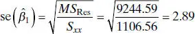
Therefore, the test statistic is

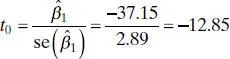
If we choose α = 0.05, the critical value of t is t 0.025,18= 2.101. Thus, we would reject H 0: β 1= 0 and conclude that there is a linear relationship between shear strength and the age of the propellant.

The Minitab output in Table 2.3 gives the standard errors of the slope and intercept (called “StDev” in the table) along with the t statistic for testing H 0: β 1= 0 and H 0: β 0= 0. Notice that the results shown in this table for the slope essentially agree with the manual calculations in Example 2.3. Like most computer software, Minitab uses the P -value approach to hypothesis testing. The P value for the test for significance of regression is reported as P = 0.000 (this is a rounded value; the actual P value is 1.64 × 10 −10). Clearly there is strong evidence that strength is linearly related to the age of the propellant. The test statistic for H 0: β 0= 0 is reported as t 0= 59.47 with P = 0.000. One would feel very confident in claiming that the intercept is not zero in this model.

We may also use an analysis-of-varianceapproach to test significance of regression. The analysis of variance is based on a partitioning of total variability in the response variable y . To obtain this partitioning, begin with the identity

(2.31)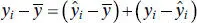

Squaring both sides of Eq. (2.31)and summing over all n observations produces

Note that the third term on the right-hand side of this expression can be rewritten as

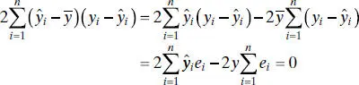
since the sum of the residuals is always zero (property 1, Section 2.2.2) and the sum of the residuals weighted by the corresponding fitted value is also zero (property 5, Section 2.2.2). Therefore,

(2.32)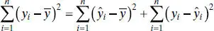

The left-hand side of Eq. (2.32)is the corrected sum of squares of the observations, SS T, which measures the total variability in the observations. The two components of SS Tmeasure, respectively, the amount of variability in the observations yi accounted for by the regression line and the residual variation left unexplained by the regression line. We recognize 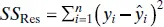as the residual or error sum of squares from Eq. (2.16). It is customary to call the regressionor model sum of squares.

Equation (2.32)is the fundamental analysis-of-variance identity for a regression model. Symbolically, we usually write

(2.33)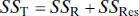

Comparing Eq. (2.33)with Eq. (2.18)we see that the regression sum of squares may be computed as

(2.34)

The degree-of-freedombreakdown is determined as follows. The total sum of squares, SS T, has df T= n − 1 degrees of freedom because one degree of freedom is lost as a result of the constraint on the deviations . The model or regression sum of squares, SS R, has df R= 1 degree of freedom because SS Ris completely determined by one parameter, namely, [see Eq. (2.34)]. Finally, we noted previously that SS Rhas df Res= n − 2 degrees of freedom because two constraints are imposed on the deviations as a result of estimating and . Note that the degrees of freedom have an additive property:

(2.35)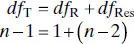

We can use the usual analysis-of-variance F test to test the hypothesis H 0: β 1= 0. Appendix C.3shows that (1) SS Res= ( n − 2) MS Res/ σ 2follows a distribution; (2) if the null hypothesis H 0: β 1= 0 is true, then SS R/ σ 2follows a distribution; and (3) SS Resand SS Rare independent. By the definition of an F statistic given in Appendix C.1,

(2.36)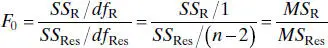

follows the F 1,n−2distribution. Appendix C.3also shows that the expected values of these mean squares are