Douglas C. Montgomery - Introduction to Linear Regression Analysis

Suppose that we wish to test the hypothesis that the slope equals a constant, say β 10. The appropriate hypotheses are

(2.23)

where we have specified a two-sided alternative. Since the errors ε i are NID(0, σ 2), the observations yi are NID( β 0+ β 1 xi , σ 2). Now is a linear combination of the observations, so is normally distributed with mean β 1and variance σ 2/ Sxx using the mean and variance of found in Section 2.2.2. Therefore, the statistic

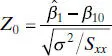
is distributed N (0, 1) if the null hypothesis H 0: β 1= β 10is true. If σ 2were known, we could use Z 0to test the hypotheses (2.23). Typically, σ 2is unknown. We have already seen that MS Resis an unbiased estimator of σ 2. Appendix C.3establishes that ( n − 2) MS Res/ σ 2follows a distribution and that MS Resand are independent. By the definition of a t statistic given in Section C.1,

(2.24)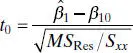

follows a t n−2distribution if the null hypothesis H 0: β 1= β 10is true. The degrees of freedom associated with t 0are the number of degrees of freedom associated with MS Res. Thus, the ratio t 0is the test statistic used to test H 0: β 1= β 10. The test procedure computes t 0and compares the observed value of t 0from Eq. (2.24)with the upper α /2 percentage point of the t n−2distribution ( t α/2,n−2). This procedure rejects the null hypothesis if

(2.25)

Alternatively, a P -value approach could also be used for decision making.

The denominator of the test statistic, t 0, in Eq. (2.24)is often called the estimated standard error, or more simply, the standard errorof the slope. That is,

(2.26)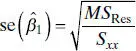

Therefore, we often see t 0written as

(2.27)

A similar procedure can be used to test hypotheses about the intercept. To test

(2.28)

we would use the test statistic

(2.29)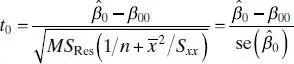

where 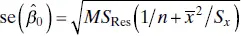is the standard error of the intercept. We reject the null hypothesis H 0: β 0= β 00if | t 0| > t α/2,n−2.

A very important special case of the hypotheses in Eq. (2.23)is

(2.30)

These hypotheses relate to the significance of regression. Failing to reject H 0: β 1= 0 implies that there is no linear relationship between x and y . This situation is illustrated in Figure 2.2. Note that this may imply either that x is of little value in explaining the variation in y and that the best estimator of y for any x is ( Figure 2.2 a ) or that the true relationship between x and y is not linear ( Figure 2.2 b ). Therefore, failing to reject H 0: β 1= 0 is equivalent to saying that there is no linear relationship between y and x.

Alternatively, if H 0: β 1= 0 is rejected, this implies that x is of value in explaining the variability in y . This is illustrated in Figure 2.3. However, rejecting H 0: β 1= 0 could mean either that the straight-line model is adequate ( Figure 2.3 a ) or that even though there is a linear effect of x , better results could be obtained with the addition of higher order polynomial terms in x ( Figure 2.3 b ).

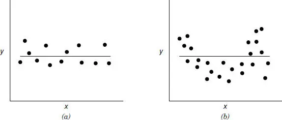
Figure 2.2 Situations where the hypothesis H 0: β 1= 0 is not rejected.

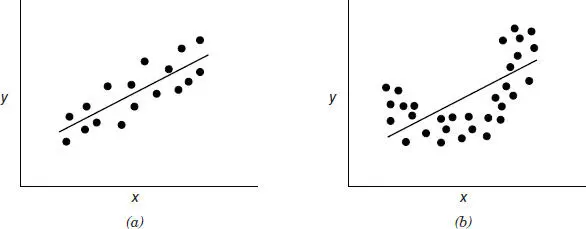
Figure 2.3 Situations where the hypothesis H 0: β 1= 0 is rejected.

The test procedure for H 0: β 1= 0 may be developed from two approaches. The first approach simply makes use of the t statistic in Eq. (2.27)with β 10= 0, or

The null hypothesis of significance of regression would be rejected if | t 0| > t α/2,n−2.

We test for significance of regression in the rocket propellant regression model of Example 2.1. The estimate of the slope is , and in Example 2.2, we computed the estimate of σ 2to be . The standard error of the slope is