Douglas C. Montgomery - Introduction to Linear Regression Analysis

(2.16)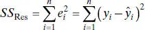

A convenient computing formula for SS Resmay be found by substituting into Eq. (2.16)and simplifying, yielding

(2.17)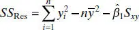

But

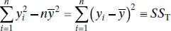
is just the corrected sum of squares of the response observations, so

(2.18)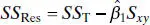

The residual sum of squares has n − 2 degrees of freedom, because two degrees of freedom are associated with the estimates and involved in obtaining . Section C.3shows that the expected value of SS Resis E ( SS Res) = ( n − 2) σ 2, so an unbiased estimator of σ2is

(2.19)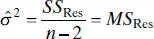

The quantity MS Resis called the residual mean square. The square root of is sometimes called the standard error of regression, and it has the same units as the response variable y .

Because depends on the residual sum of squares, any violation of the assumptions on the model errors or any misspecification of the model form may seriously damage the usefulness of as an estimate of σ 2. Because is computed from the regression model residuals, we say that it is a model-dependentestimate of σ 2.

To estimate σ 2for the rocket propellant data in Example 2.1, first find

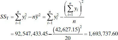
From Eq. (2.18)the residual sum of squares is

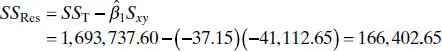
Therefore, the estimate of σ 2is computed from Eq. (2.19)as

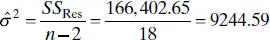
Remember that this estimate of σ 2is model dependent. Note that this differs slightly from the value given in the Minitab output (Table 2.3) because of rounding.

There is an alternate form of the simple linear regression model that is occasionally useful. Suppose that we redefine the regressor variable xi as the deviation from its own average, say . The regression model then becomes

(2.20)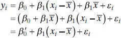

Note that redefining the regressor variable in Eq. (2.20)has shifted the origin of the x ’s from zero to . In order to keep the fitted values the same in both the original and transformed models, it is necessary to modify the original intercept. The relationship between the original and transformed intercept is

(2.21)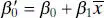

It is easy to show that the least-squares estimator of the transformed intercept is . The estimator of the slope is unaffected by the transformation. This alternate form of the model has some advantages. First, the least-squares estimators and are uncorrelated, that is, 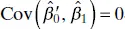. This will make some applications of the model easier, such as finding confidence intervals on the mean of y (see Section 2.4.2). Finally, the fitted model is

(2.22)

Although Eqs. (2.22)and (2.8)are equivalent (they both produce the same value of for the same value of x ), Eq. (2.22)directly reminds the analyst that the regression model is only valid over the range of x in the original data. This region is centered at .

We are often interested in testing hypotheses and constructing confidence intervals about the model parameters. Hypothesis testing is discussed in this section, and Section 2.4deals with confidence intervals. These procedures require that we make the additional assumption that the model errors εi are normally distributed. Thus, the complete assumptions are that the errors are normally and independently distributed with mean 0 and variance σ 2, abbreviated NID(0, σ 2). In Chapter 4we discuss how these assumptions can be checked through residual analysis.