Douglas C. Montgomery - Introduction to Linear Regression Analysis

(2.2a)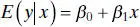

and the variance is

(2.2b)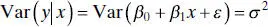

Thus, the mean of y is a linear function of x although the variance of y does not depend on the value of x . Furthermore, because the errors are uncorrelated, the responses are also uncorrelated.

The parameters β 0and β 1are usually called regression coefficients. These coefficients have a simple and often useful interpretation. The slope β 1is the change in the mean of the distribution of y produced by a unit change in x . If the range of data on x includes x = 0, then the intercept β 0is the mean of the distribution of the response y when x = 0. If the range of x does not include zero, then β 0has no practical interpretation.

The parameters β 0and β 1are unknown and must be estimated using sample data. Suppose that we have n pairs of data, say ( y 1, x 1), ( y 2, x 2), …, ( yn , xn ). As noted in Chapter 1, these data may result either from a controlled experiment designed specifically to collect the data, from an observational study, or from existing historical records (a retrospective study).

The method of least squaresis used to estimate β 0and β 1. That is, we estimate β 0and β 1so that the sum of the squares of the differences between the observations yi and the straight line is a minimum. From Eq. (2.1)we may write

(2.3)

Equation (2.1)maybe viewed as a population regression modelwhile Eq. (2.3)is a sample regression model, written in terms of the n pairs of data ( yi , xi ) ( i = 1, 2, …, n ). Thus, the least-squares criterion is

(2.4)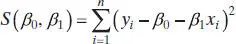

The least-squares estimators of β 0and β 1, say and , must satisfy

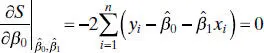
and

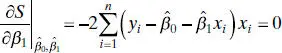
Simplifying these two equations yields

(2.5)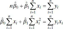

Equations (2.5)are called the least-squares normal equations. The solution to the normal equations is

(2.6)

and

(2.7)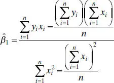

where

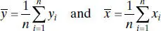
are the averages of yi and xi , respectively. Therefore, and in Eqs. (2.6)and (2.7)are the least-squares estimatorsof the intercept and slope, respectively. The fitted simple linear regression model is then

(2.8)

Equation (2.8)gives a point estimate of the mean of y for a particular x .

Since the denominator of Eq. (2.7)is the corrected sum of squares of the xi and the numerator is the corrected sum of cross products of xi and yi , we may write these quantities in a more compact notation as

(2.9)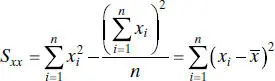

and

(2.10)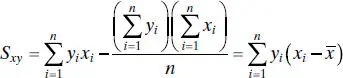

Thus, a convenient way to write Eq. (2.7)is

(2.11)

The difference between the observed value yi and the corresponding fitted value is a residual. Mathematically the i th residual is

(2.12)

Residuals play an important role in investigating model adequacyand in detecting departures from the underlying assumptions. This topic is discussed in subsequent chapters.

A rocket motor is manufactured by bonding an igniter propellant and a sustainer propellant together inside a metal housing. The shear strength of the bond between the two types of propellant is an important quality characteristic. It is suspected that shear strength is related to the age in weeks of the batch of sustainer propellant. Twenty observations on shear strength and the age of the corresponding batch of propellant have been collected and are shown in Table 2.1. The scatter diagram, shown in Figure 2.1, suggests that there is a strong statistical relationship between shear strength and propellant age, and the tentative assumption of the straight-line model y = β 0+ β 1 x + ε appears to be reasonable.