Douglas C. Montgomery - Introduction to Linear Regression Analysis
Здесь есть возможность читать онлайн «Douglas C. Montgomery - Introduction to Linear Regression Analysis» — ознакомительный отрывок электронной книги совершенно бесплатно, а после прочтения отрывка купить полную версию. В некоторых случаях можно слушать аудио, скачать через торрент в формате fb2 и присутствует краткое содержание. Жанр: unrecognised, на английском языке. Описание произведения, (предисловие) а так же отзывы посетителей доступны на портале библиотеки ЛибКат.
- Название:Introduction to Linear Regression Analysis
- Автор:
- Жанр:
- Год:неизвестен
- ISBN:нет данных
- Рейтинг книги:4 / 5. Голосов: 1
-
Избранное:Добавить в избранное
- Отзывы:
-
Ваша оценка:
Introduction to Linear Regression Analysis: краткое содержание, описание и аннотация
Предлагаем к чтению аннотацию, описание, краткое содержание или предисловие (зависит от того, что написал сам автор книги «Introduction to Linear Regression Analysis»). Если вы не нашли необходимую информацию о книге — напишите в комментариях, мы постараемся отыскать её.
New exercises and data sets New material on generalized regression techniques The inclusion of JMP software in key areas Carefully condensing the text where possible
skillfully blends theory and application in both the conventional and less common uses of regression analysis in today's cutting-edge scientific research. The text equips readers to understand the basic principles needed to apply regression model-building techniques in various fields of study, including engineering, management, and the health sciences.
Introduction to Linear Regression Analysis — читать онлайн ознакомительный отрывок
Ниже представлен текст книги, разбитый по страницам. Система сохранения места последней прочитанной страницы, позволяет с удобством читать онлайн бесплатно книгу «Introduction to Linear Regression Analysis», без необходимости каждый раз заново искать на чём Вы остановились. Поставьте закладку, и сможете в любой момент перейти на страницу, на которой закончили чтение.
Интервал:
Закладка:
TABLE 2.1 Data for Example 2.1
| Observation, i | Shear Strength, yi (psi) | Age of Propellant, xi (weeks) |
| 1 | 2158.70 | 15.50 |
| 2 | 1678.15 | 23.75 |
| 3 | 2316.00 | 8.00 |
| 4 | 2061.30 | 17.00 |
| 5 | 2207.50 | 5.50 |
| 6 | 1708.30 | 19.00 |
| 7 | 1784.70 | 24.00 |
| 8 | 2575.00 | 2.50 |
| 9 | 2357.90 | 7.50 |
| 10 | 2256.70 | 11.00 |
| 11 | 2165.20 | 13.00 |
| 12 | 2399.55 | 3.75 |
| 13 | 1779.80 | 25.00 |
| 14 | 2336.75 | 9.75 |
| 15 | 1765.30 | 22.00 |
| 16 | 2053.50 | 18.00 |
| 17 | 2414.40 | 6.00 |
| 18 | 2200.50 | 12.50 |
| 19 | 2654.20 | 2.00 |
| 20 | 1753.70 | 21.50 |
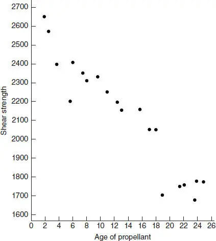
Figure 2.1 Scatter diagram of shear strength versus propellant age, Example 2.1.
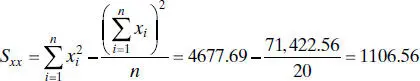
To estimate the model parameters, first calculate
and
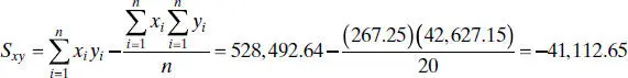
Therefore, from Eqs. (2.11)and (2.6), we find that
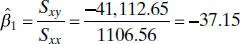
and

TABLE 2.2 Data, Fitted Values, and Residuals for Example 2.1
| Observed Value, yi | Fitted Value,  |
Residual, ei |
| 2158.70 | 2051.94 | 106.76 |
| 1678.15 | 1745.42 | −67.27 |
| 2316.00 | 2330.59 | −14.59 |
| 2061.30 | 1996.21 | 65.09 |
| 2207.50 | 2423.48 | −215.98 |
| 1708.30 | 1921.90 | −213.60 |
| 1784.70 | 1736.14 | 48.56 |
| 2575.00 | 2534.94 | 40.06 |
| 2357.90 | 2349.17 | 8.73 |
| 2256.70 | 2219.13 | 37.57 |
| 2165.20 | 2144.83 | 20.37 |
| 2399.55 | 2488.50 | −88.95 |
| 1799.80 | 1698.98 | 80.82 |
| 2336.75 | 2265.58 | 71.17 |
| 1765.30 | 1810.44 | −45.14 |
| 2053.50 | 1959.06 | 94.44 |
| 2414.40 | 2404.90 | 9.50 |
| 2200.50 | 2163.40 | 37.10 |
| 2654.20 | 2553.52 | 100.68 |
| 1753.70 | 1829.02 | −75.32 |
 |
 |
 |
The least-squares fit is
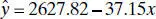
We may interpret the slope −37.15 as the average weekly decrease in propellant shear strength due to the age of the propellant. Since the lower limit of the x ’s is near the origin, the intercept 2627.82 represents the shear strength in a batch of propellant immediately following manufacture. Table 2.2 displays the observed values yi , the fitted values  , and the residuals.
After obtaining the least-squares fit, a number of interesting questions come to mind:
1 How well does this equation fit the data?
2 Is the model likely to be useful as a predictor?
3 Are any of the basic assumptions (such as constant variance and uncorrelated errors) violated, and if so, how serious is this?
All of these issues must be investigated before the model is finally adopted for use. As noted previously, the residuals play a key role in evaluating model adequacy. Residuals can be viewed as realizations of the model errors εi . Thus, to check the constant variance and uncorrelated errors assumption, we must ask ourselves if the residuals look like a random sample from a distribution with these properties. We return to these questions in Chapter 4, where the use of residuals in model adequacy checking is explored.
TABLE 2.3 Minitab Regression Output for Example 2.1
Regression Analysis |
|||||
The regression equation is |
|||||
Strength = 2628- 37.2 Age |
|||||
Predictor |
Coef |
StDev |
T |
P |
|
Constant |
2627.82 |
44.18 |
59.47 |
0.000 |
|
Age |
-37.154 |
2.889 |
-12.86 |
0.000 |
|
S = 96.11 |
R-Sq = 90.2% |
R-Sq(adj) = 89.6% |
|||
Analysis of Variance |
|||||
Source |
DF |
SS |
MS |
F |
P |
Regression |
1 |
1527483 |
1527483 |
165.38 |
0.000 |
Error |
18 |
166255 |
9236 |
||
Total |
19 |
1693738 |
Computer Output
Computer software packages are used extensively in fitting regression models. Regression routines are found in both network and PC-based statistical software, as well as in many popular spreadsheet packages. Table 2.3 presents the output from Minitab, a widely used PC-based statistics package, for the rocket propellant data in Example 2.1. The upper portion of the table contains the fitted regression model. Notice that before rounding the regression coefficients agree with those we calculated manually. Table 2.3 also contains other information about the regression model. We return to this output and explain these quantities in subsequent sections.
Читать дальшеИнтервал:
Закладка:
Похожие книги на «Introduction to Linear Regression Analysis»
Представляем Вашему вниманию похожие книги на «Introduction to Linear Regression Analysis» списком для выбора. Мы отобрали схожую по названию и смыслу литературу в надежде предоставить читателям больше вариантов отыскать новые, интересные, ещё непрочитанные произведения.


Обсуждение, отзывы о книге «Introduction to Linear Regression Analysis» и просто собственные мнения читателей. Оставьте ваши комментарии, напишите, что Вы думаете о произведении, его смысле или главных героях. Укажите что конкретно понравилось, а что нет, и почему Вы так считаете.