Douglas C. Montgomery - Introduction to Linear Regression Analysis
Здесь есть возможность читать онлайн «Douglas C. Montgomery - Introduction to Linear Regression Analysis» — ознакомительный отрывок электронной книги совершенно бесплатно, а после прочтения отрывка купить полную версию. В некоторых случаях можно слушать аудио, скачать через торрент в формате fb2 и присутствует краткое содержание. Жанр: unrecognised, на английском языке. Описание произведения, (предисловие) а так же отзывы посетителей доступны на портале библиотеки ЛибКат.
- Название:Introduction to Linear Regression Analysis
- Автор:
- Жанр:
- Год:неизвестен
- ISBN:нет данных
- Рейтинг книги:4 / 5. Голосов: 1
-
Избранное:Добавить в избранное
- Отзывы:
-
Ваша оценка:
Introduction to Linear Regression Analysis: краткое содержание, описание и аннотация
Предлагаем к чтению аннотацию, описание, краткое содержание или предисловие (зависит от того, что написал сам автор книги «Introduction to Linear Regression Analysis»). Если вы не нашли необходимую информацию о книге — напишите в комментариях, мы постараемся отыскать её.
New exercises and data sets New material on generalized regression techniques The inclusion of JMP software in key areas Carefully condensing the text where possible
skillfully blends theory and application in both the conventional and less common uses of regression analysis in today's cutting-edge scientific research. The text equips readers to understand the basic principles needed to apply regression model-building techniques in various fields of study, including engineering, management, and the health sciences.
Introduction to Linear Regression Analysis — читать онлайн ознакомительный отрывок
Ниже представлен текст книги, разбитый по страницам. Система сохранения места последней прочитанной страницы, позволяет с удобством читать онлайн бесплатно книгу «Introduction to Linear Regression Analysis», без необходимости каждый раз заново искать на чём Вы остановились. Поставьте закладку, и сможете в любой момент перейти на страницу, на которой закончили чтение.
Интервал:
Закладка:
For the distillation example, a very reasonable experimental strategy uses every possible treatment combination to form a basic experiment with eight different settings for the process. Table 1.1 presents these combinations of high and low levels. This experimental arrangement is called a factorial design.
Figure 1.7illustrates that this factorial design forms a cube in terms of these high and low levels. With each setting of the process conditions, we allow the column to reach equilibrium, take a sample of the product stream, and determine the acetone concentration. We then can draw specific inferences about the effect of these factors. Such an approach allows us to proactively study a population or process.
TABLE 1.1 Designed Experiment for the Distillation Column
| Reboil Temperature | Condensate Temperature | Reflux Rate |
| −1 | −1 | −1 |
| +1 | −1 | −1 |
| −1 | +1 | −1 |
| +1 | +1 | −1 |
| −1 | −1 | +1 |
| +1 | −1 | +1 |
| −1 | +1 | +1 |
| +1 | +1 | +1 |
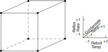
Figure 1.7 The designed experiment for the distillation column.
1.3 USES OF REGRESSION
Regression models are used for several purposes, including the following:
1 Data description
2 Parameter estimation
3 Prediction and estimation
4 Control
Engineers and scientists frequently use equations to summarize or describe a set of data. Regression analysis is helpful in developing such equations. For example, we may collect a considerable amount of delivery time and delivery volume data, and a regression model would probably be a much more convenient and useful summary of those data than a table or even a graph.
Sometimes parameter estimation problems can be solved by regression methods. For example, chemical engineers use the Michaelis–Menten equation y = β 1 x /( x + β 2) + ε to describe the relationship between the velocity of reaction y and concentration x . Now in this model, β 1is the asymptotic velocity of the reaction, that is, the maximum velocity as the concentration gets large. If a sample of observed values of velocity at different concentrations is available, then the engineer can use regression analysis to fit this model to the data, producing an estimate of the maximum velocity. We show how to fit regression models of this type in Chapter 12.
Many applications of regression involve prediction of the response variable. For example, we may wish to predict delivery time for a specified number of cases of soft drinks to be delivered. These predictions may be helpful in planning delivery activities such as routing and scheduling or in evaluating the productivity of delivery operations. The dangers of extrapolation when using a regression model for prediction because of model or equation error have been discussed previously (see Figure 1.5). However, even when the model form is correct, poor estimates of the model parameters may still cause poor prediction performance.
Regression models may be used for control purposes. For example, a chemical engineer could use regression analysis to develop a model relating the tensile strength of paper to the hardwood concentration in the pulp. This equation could then be used to control the strength to suitable values by varying the level of hardwood concentration. When a regression equation is used for control purposes, it is important that the variables be related in a causal manner. Note that a cause-and-effect relationship may not be necessary if the equation is to be used only for prediction. In this case it is only necessary that the relationships that existed in the original data used to build the regression equation are still valid. For example, the daily electricity consumption during August in Atlanta, Georgia, may be a good predictor for the maximum daily temperature in August. However, any attempt to reduce the maximum temperature by curtailing electricity consumption is clearly doomed to failure.
1.4 ROLE OF THE COMPUTER
Building a regression model is an iterative process. The model-building process is illustrated in Figure 1.8. It begins by using any theoretical knowledge of the process that is being studied and available data to specify an initial regression model. Graphical data displays are often very useful in specifying the initial model. Then the parameters of the model are estimated, typically by either least squares or maximum likelihood. These procedures are discussed extensively in the text. Then model adequacy must be evaluated. This consists of looking for potential misspecification of the model form, failure to include important variables, including unnecessary variables, or unusual/inappropriate data. If the model is inadequate, then adjustments must be made and the parameters estimated again. This process may be repeated several times until an adequate model is obtained. Finally, model validation should be carried out to ensure that the model will produce results that are acceptable in the final application.
A good regression computer program is a necessary tool in the model-building process. However, the routine application of standard regression computer programs often does not lead to successful results. The computer is nota substitute for creative thinking about the problem. Regression analysis requires the intelligentand artfuluse of the computer. We must learn how to interpret what the computer is telling us and how to incorporate that information in subsequent models. Generally, regression computer programs are part of more general statistics software packages, such as Minitab, SAS, JMP, and R. We discuss and illustrate the use of these packages throughout the book. Appendix Dcontains details of the SAS procedures typically used in regression modeling along with basic instructions for their use. Appendix Eprovides a brief introduction to the R statistical software package. We present R code for doing analyses throughout the text. Without these skills, it is virtually impossible to successfully build a regression model.
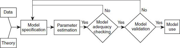
Figure 1.8 Regression model-building process.
CHAPTER 2
SIMPLE LINEAR REGRESSION
2.1 SIMPLE LINEAR REGRESSION MODEL
This chapter considers the simple linear regression model, that is, a model with a single regressor x that has a relationship with a response y that is a straight line. This simple linear regression model is
(2.1) 
where the intercept β 0and the slope β 1are unknown constants and ε is a random error component. The errors are assumed to have mean zero and unknown variance σ 2. Additionally we usually assume that the errors are uncorrelated. This means that the value of one error does not depend on the value of any other error.
It is convenient to view the regressor x as controlled by the data analyst and measured with negligible error, while the response y is a random variable. That is, there is a probability distribution for y at each possible value for x . The mean of this distribution is
Читать дальшеИнтервал:
Закладка:
Похожие книги на «Introduction to Linear Regression Analysis»
Представляем Вашему вниманию похожие книги на «Introduction to Linear Regression Analysis» списком для выбора. Мы отобрали схожую по названию и смыслу литературу в надежде предоставить читателям больше вариантов отыскать новые, интересные, ещё непрочитанные произведения.


Обсуждение, отзывы о книге «Introduction to Linear Regression Analysis» и просто собственные мнения читателей. Оставьте ваши комментарии, напишите, что Вы думаете о произведении, его смысле или главных героях. Укажите что конкретно понравилось, а что нет, и почему Вы так считаете.