Douglas C. Montgomery - Introduction to Linear Regression Analysis

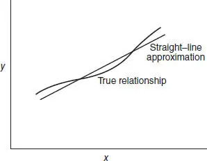
Figure 1.3 Linear regression approximation of a complex relationship.

For example, suppose that the true regression model relating delivery time to delivery volume is μ y|x= 3.5 + 2 x , and suppose that the variance is σ 2= 2. Figure 1.2illustrates this situation. Notice that we have used a normal distribution to describe the random variation in ε . Since y is the sum of a constant β 0+ β 1 x (the mean) and a normally distributed random variable, y is a normally distributed random variable. For example, if x = 10 cases, then delivery time y has a normal distribution with mean 3.5 + 2(10) = 23.5 minutes and variance 2. The variance σ 2determines the amount of variability or noise in the observations y on delivery time. When σ 2is small, the observed values of delivery time will fall close to the line, and when σ 2is large, the observed values of delivery time may deviate considerably from the line.

In almost all applications of regression, the regression equation is only an approximation to the true functional relationship between the variables of interest. These functional relationships are often based on physical, chemical, or other engineering or scientific theory, that is, knowledge of the underlying mechanism. Consequently, these types of models are often called mechanistic models. For example, the familiar physics equation momentum = mass × velocity is a mechanistic model.

Regression models, on the other hand, are thought of as empirical models. Figure 1.3illustrates a situation where the true relationship between y and x is relatively complex, yet it may be approximated quite well by a linear regression equation. Sometimes the underlying mechanism is more complex, resulting in the need for a more complex approximating function, as in Figure 1.4, where a “piecewise linear” regression function is used to approximate the true relationship between y and x .

Generally regression equations are valid only over the region of the regressor variables contained in the observed data. For example, consider Figure 1.5. Suppose that data on y and x were collected in the interval x 1≤ x ≤ x 2. Over this interval the linear regression equation shown in Figure 1.5is a good approximation of the true relationship. However, suppose this equation were used to predict values of y for values of the regressor variable in the region x 2≤ x ≤ x 3. Clearly the linear regression model is not going to perform well over this range of x because of model error or equation error.

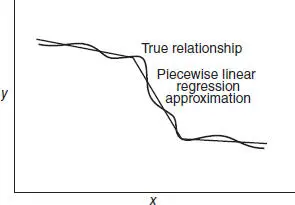
Figure 1.4 Piecewise linear approximation of a complex relationship.

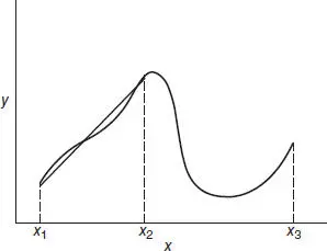
Figure 1.5 The danger of extrapolation in regression.

In general, the response variable y may be related to k regressors, x 1, x 2, …, xk , so that

(1.3)

This is called a multiple linear regression modelbecause more than one regressor is involved. The adjective linear is employed to indicate that the model is linear in the parameters β 0, β 1, …, βk , not because y is a linear function of the x ’s. We shall see subsequently that many models in which y is related to the x ’s in a nonlinear fashion can still be treated as linear regression models as long as the equation is linear in the β ’s.

An important objective of regression analysis is to estimate the unknown parametersin the regression model. This process is also called fitting the model to the data. We study several parameter estimation techniques in this book. One of these techmques is the method of least squares (introduced in Chapter 2). For example, the least-squares fit to the delivery time data is

where is the fitted or estimated value of delivery time corresponding to a delivery volume of x cases. This fitted equation is plotted in Figure 1.1 b .

The next phase of a regression analysis is called model adequacy checking, in which the appropriateness of the model is studied and the quality of the fit ascertained. Through such analyses the usefulness of the regression model may be determined. The outcome of adequacy checking may indicate either that the model is reasonable or that the original fit must be modified. Thus, regression analysis is an iterativeprocedure, in which data lead to a model and a fit of the model to the data is produced. The quality of the fit is then investigated, leading either to modification of the model or the fit or to adoption of the model. This process is illustrated several times in subsequent chapters.

A regression model does not imply a cause-and-effect relationship between the variables. Even though a strong empirical relationship may exist between two or more variables, this cannot be considered evidence that the regressor variables and the response are related in a cause-and-effect manner. To establish causality, the relationship between the regressors and the response must have a basis outside the sample data—for example, the relationship may be suggested by theoretical considerations. Regression analysis can aid in confirming a cause-and-effect relationship, but it cannot be the sole basis of such a claim.

Finally it is important to remember that regression analysis is part of a broader data-analytic approach to problem solving. That is, the regression equation itself may not be the primary objective of the study. It is usually more important to gain insight and understanding concerning the system generating the data.

An essential aspect of regression analysis is data collection. Any regression analysis is only as good as the data on which it is based. Three basic methods for collecting data are as follows:

A retrospective study based on historical data

An observational study

A designed experiment

A good data collection scheme can ensure a simplified and a generally more applicable model. A poor data collection scheme can result in serious problems for the analysis and its interpretation. The following example illustrates these three methods.

Consider the acetone–butyl alcohol distillation column shown in Figure 1.6. The operating personnel are interested in the concentration of acetone in the distillate (product) stream. Factors that may influence this are the reboil temperature, the condensate temperature, and the reflux rate. For this column, operating personnel maintain and archive the following records: