Douglas C. Montgomery - Introduction to Linear Regression Analysis
Здесь есть возможность читать онлайн «Douglas C. Montgomery - Introduction to Linear Regression Analysis» — ознакомительный отрывок электронной книги совершенно бесплатно, а после прочтения отрывка купить полную версию. В некоторых случаях можно слушать аудио, скачать через торрент в формате fb2 и присутствует краткое содержание. Жанр: unrecognised, на английском языке. Описание произведения, (предисловие) а так же отзывы посетителей доступны на портале библиотеки ЛибКат.
- Название:Introduction to Linear Regression Analysis
- Автор:
- Жанр:
- Год:неизвестен
- ISBN:нет данных
- Рейтинг книги:4 / 5. Голосов: 1
-
Избранное:Добавить в избранное
- Отзывы:
-
Ваша оценка:
Introduction to Linear Regression Analysis: краткое содержание, описание и аннотация
Предлагаем к чтению аннотацию, описание, краткое содержание или предисловие (зависит от того, что написал сам автор книги «Introduction to Linear Regression Analysis»). Если вы не нашли необходимую информацию о книге — напишите в комментариях, мы постараемся отыскать её.
New exercises and data sets New material on generalized regression techniques The inclusion of JMP software in key areas Carefully condensing the text where possible
skillfully blends theory and application in both the conventional and less common uses of regression analysis in today's cutting-edge scientific research. The text equips readers to understand the basic principles needed to apply regression model-building techniques in various fields of study, including engineering, management, and the health sciences.
Introduction to Linear Regression Analysis — читать онлайн ознакомительный отрывок
Ниже представлен текст книги, разбитый по страницам. Система сохранения места последней прочитанной страницы, позволяет с удобством читать онлайн бесплатно книгу «Introduction to Linear Regression Analysis», без необходимости каждый раз заново искать на чём Вы остановились. Поставьте закладку, и сможете в любой момент перейти на страницу, на которой закончили чтение.
Интервал:
Закладка:
Figure 2.5shows the 95% prediction interval calculated from (2.45)for the rocket propellant regression model. Also shown on this graph is the 95% CI on the mean [that is, E ( y | x ) from Eq. (2.43). This graph nicely illustrates the point that the prediction interval is wider than the corresponding CI.
We may generalize (2.45)somewhat to find a 100(1 − α ) percent prediction interval on the meanof m future observations on the response at x = x 0. Let  be the mean of m future observations at x = x 0. A point estimator of
  is
is 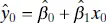 . The 100(1 − α )% prediction interval on
  is
is
(2.46) 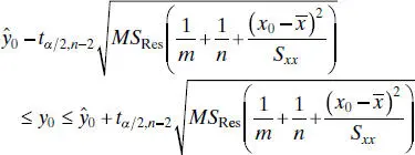
2.6 COEFFICIENT OF DETERMINATION
The quantity
(2.47) 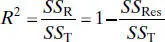
is called the coefficient of determination. Since SS Tis a measure of the variability in y without considering the effect of the regressor variable x and SS Resis a measure of the variability in y remaining after x has been considered, R 2is often called the proportion of variation explained by the regressor x . Because 0 ≤ SS Res≤ SS T, it follows that 0 ≤ R 2≤ 1. Values of R 2that are close to 1 imply that most of the variability in y is explained by the regression model. For the regression model for the rocket propellant data in Example 2.1, we have
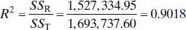
that is, 90.18% of the variability in strength is accounted for by the regression model.
The statistic R 2should be used with caution, since it is always possible to make R 2large by adding enough terms to the model. For example, if there are no repeat points (more than one y value at the same x value), a polynomial of degree n − 1 will give a “perfect” fit ( R 2= 1) to n data points. When there are repeat points, R 2can never be exactly equal to 1 because the model cannot explain the variability related to “pure” error.
Although R 2cannot decrease if we add a regressor variable to the model, this does not necessarily mean the new model is superior to the old one. Unless the error sum of squares in the new model is reduced by an amount equal to the original error mean square, the new model will have a larger error mean square than the old one because of the loss of one degree of freedom for error. Thus, the new model will actually be worse than the old one.
The magnitude of R 2also depends on the range of variability in the regressor variable. Generally R 2will increase as the spread of the x ’s increases and decrease as the spread of the x ’s decreases provided the assumed model form is correct. By the delta method (also see Hahn 1973), one can show that the expected value of R 2from a straight-line regression is approximately
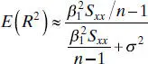
Clearly the expected value of R 2will increase (decrease) as Sxx (a measure of the spread of the x ’s) increases (decreases). Thus, a large value of R 2may result simply because x has been varied over an unrealistically large range. On the other hand, R 2may be small because the range of x was too small to allow its relationship with y to be detected.
There are several other misconceptions about R 2. In general, R 2does not measure the magnitude of the slope of the regression line. A large value of R 2does not imply a steep slope. Furthermore, R 2does not measure the appropriateness of the linear model, for R 2will often be large even though y and x are nonlinearly related. For example, R 2for the regression equation in Figure 2.3 b will be relatively large even though the linear approximation is poor. Remember that although R 2is large, this does not necessarily imply that the regression model will be an accurate predictor.
2.7 A SERVICE INDUSTRY APPLICATION OF REGRESSION
A hospital is implementing a program to improve service quality and productivity. As part of this program the hospital management is attempting to measure and evaluate patient satisfaction. Table B.17 contains some of the data that have been collected on a random sample of 25 recently discharged patients. The response variable is satisfaction, a subjective response measure on an increasing scale. The potential regressor variables are patient age, severity (an index measuring the severity of the patient’s illness), an indicator of whether the patient is a surgical or medical patient (0 = surgical, 1 = medical), and an index measuring the patient’s anxiety level. We start by building a simple linear regression model relating the response variable satisfaction to severity.
Figure 2.6is a scatter diagram of satisfaction versus severity. There is a relatively mild indication of a potential linear relationship between these two variables. The output from JMP for fitting a simple linear regression model to these data is shown in Figure 2.7. JMP is an SAS product that is a menu-based PC statistics package with an extensive array of regression modeling and analysis capabilities.
At the top of the JMP output is the scatter plot of the satisfaction and severity data, along with the fitted regression line. The straight line fit looks reasonable although there is considerable variability in the observations around the regression line. The second plot is a graph of the actual satisfaction response versus the predicted response. If the model were a perfect fit to the data all of the points in this plot would lie exactly along the 45-degree line. Clearly, this model does not provide a perfect fit. Also, notice that while the regressor variable is significant (the ANOVA F statistic is 17.1114 with a P value that is less than 0.0004), the coefficient of determination R 2= 0.43. That is, the model only accounts for about 43% of the variability in the data. It can be shown by the methods discussed in Chapter 4that there are no fundamental problems with the underlying assumptions or measures of model adequacy, other than the rather low value of R 2.
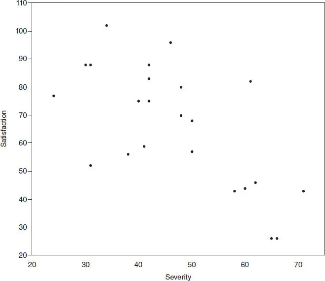
Figure 2.6 Scatter diagram of satisfaction versus severity.
Читать дальшеИнтервал:
Закладка:
Похожие книги на «Introduction to Linear Regression Analysis»
Представляем Вашему вниманию похожие книги на «Introduction to Linear Regression Analysis» списком для выбора. Мы отобрали схожую по названию и смыслу литературу в надежде предоставить читателям больше вариантов отыскать новые, интересные, ещё непрочитанные произведения.


Обсуждение, отзывы о книге «Introduction to Linear Regression Analysis» и просто собственные мнения читателей. Оставьте ваши комментарии, напишите, что Вы думаете о произведении, его смысле или главных героях. Укажите что конкретно понравилось, а что нет, и почему Вы так считаете.